9 Tutorial: Introduction to R Markdown
After working through Tutorial 9, you’ll…
- know how to set up RMarkdown and Zotero
- know RMarkdown syntax to write papers in R
R Markdown is a powerful tool for scientists that allows you to intermingle code and text in a single document. It’s a versatile R package that combines the core syntax of markdown (an easy-to-write plain text format) with embedded R code chunks, enabling the creation of dynamic documents, presentations, dashboards, and even entire books (R Markdown supports a variety of output formats, including HTML, PDF, Microsoft Word and MANY more!).
Developed by Yihui Xie in 2012, and actively maintained by the RStudio team, R Markdown was designed to provide a workflow for both data analysis and reporting. One of the key features of R Markdown is its ability to execute R code chunks in the document and automatically capture the output and include it in the final document. This can include results of computations, tables, and even graphics generated by the R code. R Markdown documents are completely reproducible and can be automatically regenerated whenever the underlying data or analysis code changes.
Creating an R Markdown document is an interactive process that combines elements of coding, data analysis, and scientific writing. Let’s get started.
9.1 Packages
Firstly, you’ll need to install the rmarkdown package and its
dependencies, including knitr for executing code chunks. You can do
this from within R or RStudio:
# install.packages("rmarkdown") # run only the first time
# install.packages("knitr") # run only the first timeIn addition, you’ll need a LaTeX installation on your PC / Mac. Some of you might already have installed LaTeX, such as in MiKTeX on Windows. If you don’t, please install tinytex in R:
We are all clear. Let’s get started!
9.2 Creating a new R Markdown file
You can create a new R Markdown file in RStudio by clicking on
File > New File > R Markdown... This will open a dialog box where you
can give the document a title and author, and choose the output format
(HTML, PDF, or Word).
Let’s choose “PDF” and provide the title “My first R Markdown document”.
9.3 Structure of R Markdown documents
An R Markdown document consists of YAML metadata, markdown text, and R code chunks.
YAML Metadata: This is the section at the top of the document, enclosed in
- - -. It contains information like the title, author, date, and output format of the document.Markdown Text: Markdown is a simple formatting syntax that allows you to include things like headers, links, italics, bullet lists, images, etc., in plain text.
R Code Chunks: You can insert R code into your document by enclosing it in
```{r} ```.
This code chunk will be executed when the document is rendered. Let’s test it in the next chapter.
9.4 Rendering the document
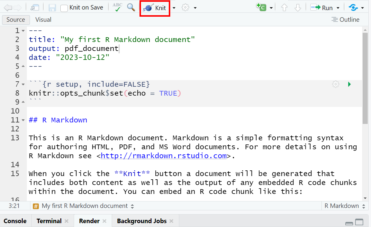
Our new RMarkdown document, which you’ve titled “My first R Markdown document”, already includes pre-prepared text and code. To render the document, click on the Knit button (represented by the yarn symbol with a needle) found within your RMarkdown (Rmd) script.
| How to knit (i.e., render) an RMarkdown document |
 |
If you haven’t saved your RMarkdown (Rmd) script yet, you will be prompted to do so before knitting. In such a case, save your script in your current working directory under the name "my_rmarkdown_document.Rmd" and click knit again.
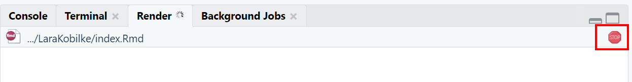
During the knitting process, you’ll see a red stop sign on the right-hand side of your console. This indicates that the R compiler is still processing. Once the stop sign disappears, you’ll find a neatly rendered PDF document in your working directory.
| How to know when the knitting process is finished: Keep an eye on the stop sign |
 |
If you don’t like to use the knit button, you can also use the render() function from the rmarkdown package to render / knit your document:
This will execute all of the R code chunks, convert the markdown text to formatted text, and combine everything into a final PDF document that is saved to your working directory.
9.5 Formatting the document
You can format your R Markdown document by using Markdown as a simple formatting syntax. This is the basic syntax:
Headers: Use # for a top-level header (H1), ## for H2, up to ###### for H6. The more #s, the smaller the header.
Emphasis: For italic text, wrap words in * or _ , like * italic * or _ italic _ . For bold, use double ** or __ , like ** bold ** or __ bold __.
Lists: Use *, -, or + followed by a space for bullet points. For numbered items, start the line with the number, a period, and a space.
Links: Wrap the clickable text in square brackets [] and the URL in parentheses (), like this but without the space:
[Lara Kobike] (homepage_url).Images: Similar to links, but prefix the square bracket with an exclamation point !, like this but without the space:
![] (image_url).Code: Use backticks ` around inline code snippets. For larger blocks of code, use triple backticks.
Blockquotes: Start the line with a > to create a blockquote.
Footnotes: The footnote number is placed inside the square bracket after a caret:
^[ 4 ]. Then you put the text of the footnote after another caret:^[ 4 ]: This is how a footnote looks like after rendering.4
Finally, you can use this R Markdown cheat sheet to quickly learn more.
Tip for advanced users: The bookdown package extends the functionality of the rmarkdown package. It can be used to create long and more complicated documents. Here is an introduction to bookdown by Benjamin Fretwurst, which he created for his students in Zurich (including videos): Link.”
9.6 Citing papers with Zotero
You can integrate Zotero to cite your sources within an R Markdown document. Watch my video where I set up this ecosystem on my PC, following this tutorial:
First, you need to download and install Zotero. It’s a free, open-source tool that helps you collect, organize, cite, and share your research sources. After you have Zotero installed, you also need to install an extension called Better BibTeX for Zotero, which simplifies the process of exporting your Zotero libraries in a format that is easy to use with R Markdown.
To install Better BibTeX, open Zotero and follow this path:
Tools > Add-Ons > Gear Icon > Install Add-On From File…. Then go to
the folder you downloaded the Better Bibtex file to. Select the
BetterBibtex.xpi file, click “Install Now” in the Zotero pop-up, and
follow the system setup.
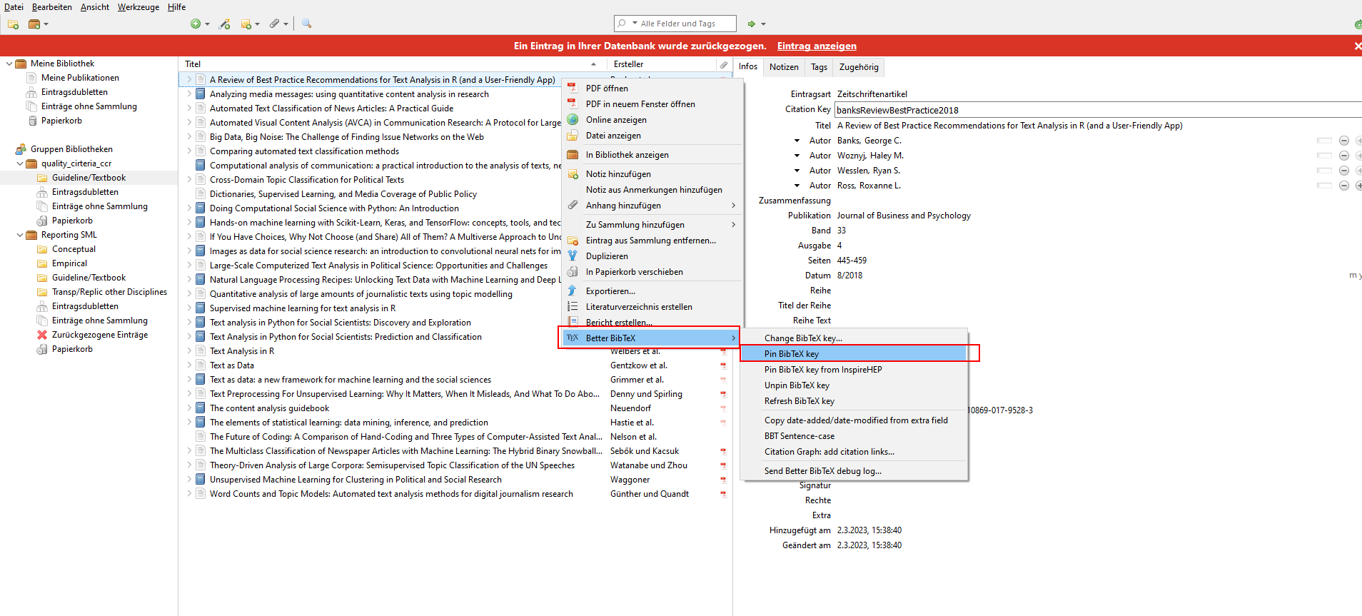
Tip for advanced users: Better BibTeX will create dynamic citation keys from the Zotero paper information, and this key may change when you edit the paper in Zotero. You can generate a pinned (i.e., fixed) citation key by selecting one or more items, right-clicking, and selecting Pin BibTeX key, which will add the current citation key to the “extra” field, thereby pinning it. If you want to update your citation key default style, go to Tools > Better BibTex > Open Better BibTex Preferences and enter your desired citation key style, e.g. “auth.fold.lower + year”. See this screenshot for a visual aid:
| How to pin BibTex keys in Zotero: |
 |
Next, you need to connect Zotero with R Markdown. The easiest way that
I’ve found is through using the rbbt package (see the author’s blog
here).
However, it’s not hosted on CRAN, so be careful. This package might
not run stable in the future.
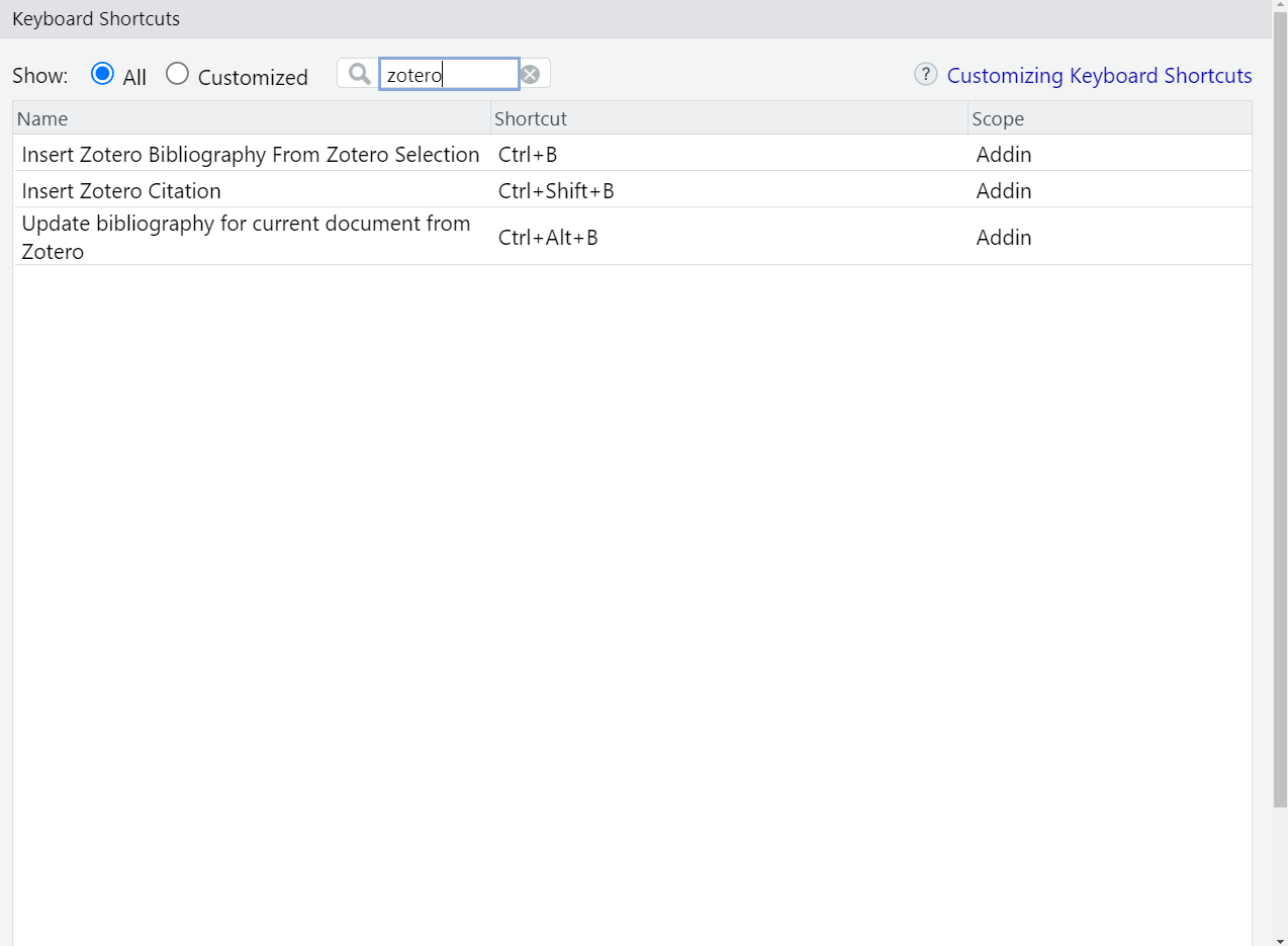
After installing rbbt and restarting RStudio, go to
Tools > Modify Keyboard Shortcuts. Search for zotero and click on
the ‘Shortcut’ field for the ‘Insert Zotero Bibliography from Zotero
Selection’ line and type in your desired shortcut keys, e.g.
CNTRL + B. See this screenshot for a visual aid:
| How to modify your Zotero BibTex Shortcuts in RStudio: |
 |
Alright, now it’s time to open a new R script. Go to
File > New File > R Script and open an empty document. Save this
document via File > Save As and call it “references.bib”. You will see
a warning that this is changing the R script to be a bib file. This
warning is great news because that’s exactly what we want. Make sure
that your references.bib is placed in the same directory as your R
Markdown .Rmd file.
Next, switch to Zotero and select all references that you want to cite.
For example, use the shortcut CNTRL + A in your Zotero project to
select all papers in that project at the same time. Move back to R
Markdown and into your “references.bib” file. Go in there and hit your
‘Insert Zotero Bibliography from Zotero Selection’ shortcut (i.e.
CNTRL + B). Voilá, you got yourself a bibliography to cite from that
you can always easily update using CNTRL + B. Save that updated .bib
file.
In the R Markdown .Rmd file, we add to following line to the end of your YAML header:
bibliography: references.bib
Now, whenever you are in your R Markdown file, you can just type an “@” symbol and RStudio will automatically prompt you with the options from your .bib file. Choose your reference and hit Enter. This will insert the citation key in your R Markdown document, e.g. @smith2023. In the actual output, @smith2023 will be replaced by a properly formatted citation, and a reference list will be automatically generated at the end of your document.
Here’s an overview of all citekeys in RMarkdown:
| Citekeys in RMarkdown: |
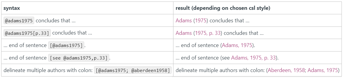 |
For more details on how to use Zotero with R Markdown, including how to specify citation style and how to cite page numbers, see the official guide on using Zotero with R Markdown.
9.7 Basic setup of an Rmd script
Every R(md) script has a similar setup: You load libraries, set some global options, define your working directory, load data, manipulate data and run analyses. In this part of the tutorial, we will turn your my-rmarkdown-document.Rmd into a template for R script setup.
To do this, we’ll first delete all R Markdown text and create an empty document like this:
| Clear your Rmd script: |
Now we are ready to fill your template document!
- Update your YAML header with APA7 information:
Install and load the
papajapackage, which allows to create APA7-styled papers:
If you want to use the most recent (development!) version of papaja that supports APA7, follow this tutorial and install from GitHub: remotes::install_github("crsh/papaja@devel")
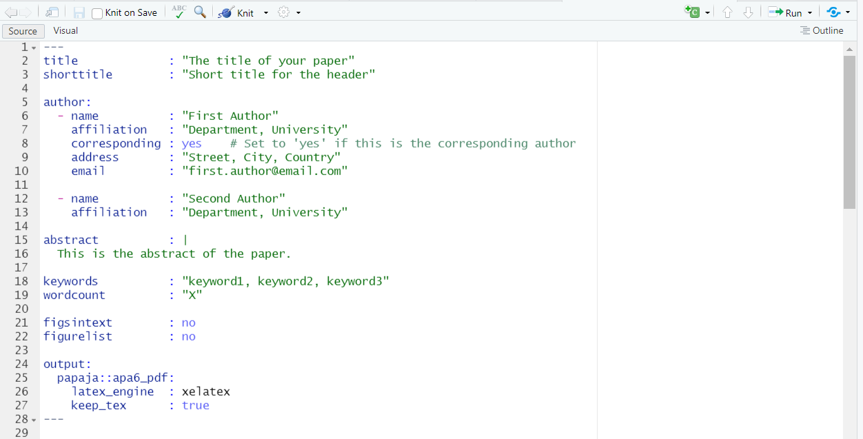
Next, copy and paste this new YAML header into your Rmd file:
title             : "The title of your paper"
shorttitle        : "Short title for the header"

author:
  - name          : "First Author"
    affiliation   : "Department, University"
    corresponding : yes    # Set to 'yes' if this is the corresponding author
    address       : "Street, City, Country"
    email         : "first.author@email.com"

  - name          : "Second Author"
    affiliation   : "Department, University"

abstract          : |
  This is the abstract of the paper.

keywords          : "keyword1, keyword2, keyword3"
wordcount         : "X"

figsintext        : no
figurelist        : no

output:
  papaja::apa6_pdf:
    latex_engine  : xelatex
    keep_tex      : true
---
This is what your Rmd document should look like:
| Set up a APA7 YAML header in Rmd: |
 |
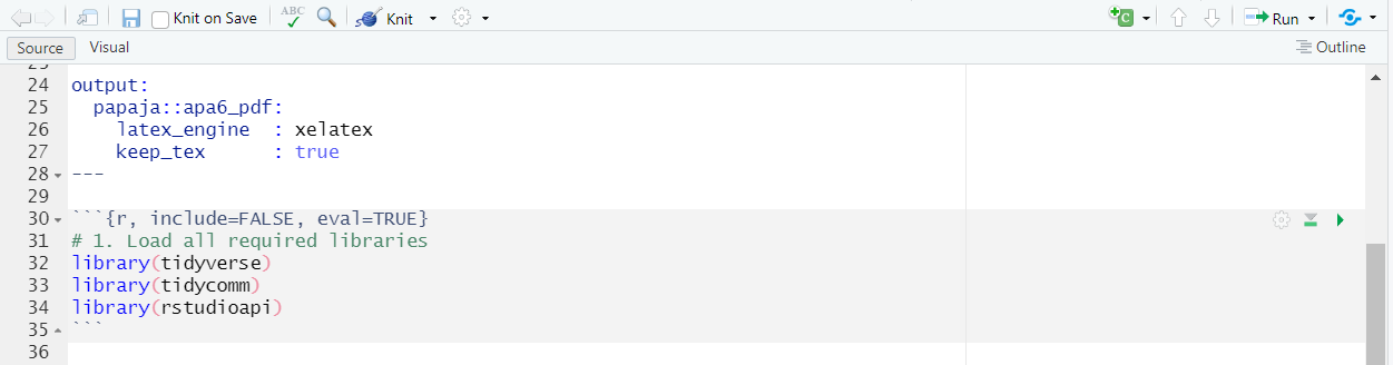
- Load libraries: It’s customary to start your script by loading the required libraries. These are be some of the libraries that you might like to use:
This is what your Rmd document should look like:
| Set up your libraries in Rmd: |
 |
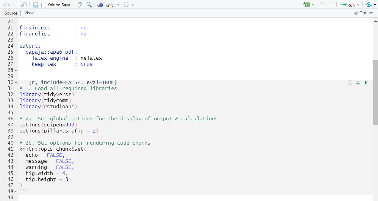
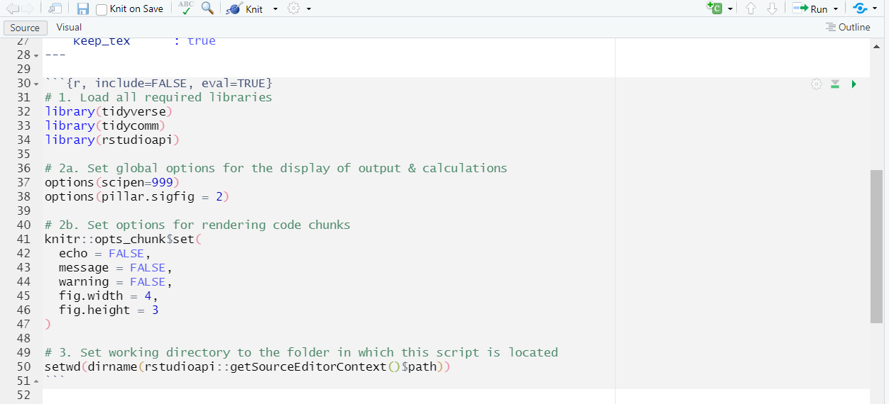
- Setting global options At times, you’ll want to establish certain options that apply throughout your R(md) file. You’ve already learned about these options in the tutorial: Optional: Setting global options in R for a customized workflow.
# Set global options for the display of output & calculations
options(scipen=999) # turns off scientific notation
options(pillar.sigfig = 2) # desired number of decimal points in tibbles
In addition to setting these global options for displaying output in tibbles, you may also want to control how your code chunks render in the PDF. For example, you might wish to set the size of figures that appear in your rendered document:
# Set options for rendering code chunks
knitr::opts_chunk$set(
  echo = TRUE,         # show code in output, this is usually turned off when you hand in your publications for review
  message = FALSE,     # suppress messages (the smaller siblings of warnings that give you additional information on your console output)
  warning = FALSE,     # suppress all warnings
  fig.width = 6,       # figure width in inch
  fig.height = 4       # figure height in inch
  )
This is what your Rmd document should look like:
| Set up your options in Rmd: |
 |
- Setting the working directory Next, set your working directory with soft coding:
This is what your Rmd document should look like:
| Set up your working directory in Rmd: |
 |
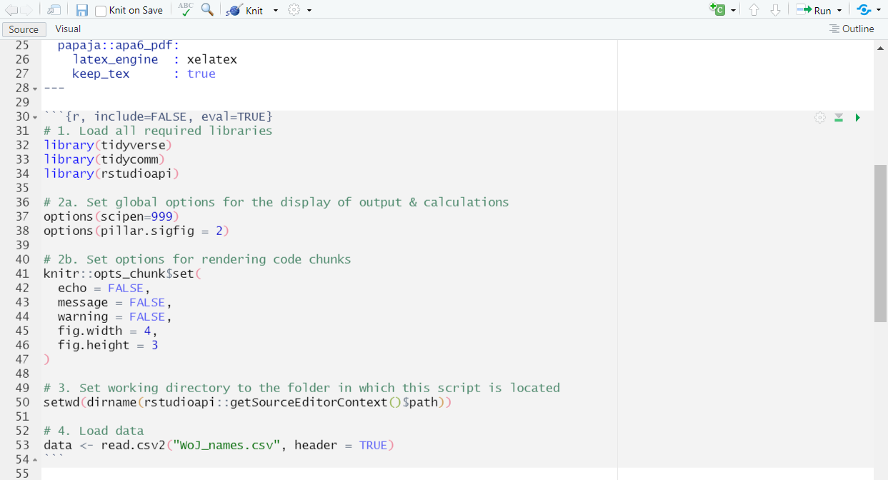
- Load data: Now, you’ll load your data from your working directory.
This is what your Rmd document should look like:
| Load data in Rmd: |
 |
- Write content: We made it to the end of this tutorial! This is were you can start writing your fully reproducible paper! :) You can write stuff like this:
With this preamble, we are all set. You can write your paper here using R Markdown syntax.
# Theory
This is my theory section.
## Sub-Theory 1
This is the first sub-section of my theory section.
## Sub-Theory 2
This is the second sub-section of my theory section.
# Method
This is my method section. But I need to refer back to my [Theory] section to show you how to do it. In addition, I'll set this [link](https://www.ifkw.uni-muenchen.de/index.html) to our department's website. Really strange method section.
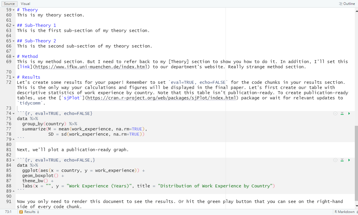
# Results
Let's create some results for your paper! Remember to set `eval=TRUE, echo=FALSE` for the code chunks in your results section. This is the only way your calculations and figures will be displayed in the final paper. Let's first create our table with descriptive statistics of work experience by country. Note that this table isn't publication-ready. To create publication-ready tables, use the [`sjPlot`](https://cran.r-project.org/web/packages/sjPlot/index.html) package or wait for relevant updates to `tidycomm`.
{r, eval=TRUE, echo=FALSE} data %>% group_by(country) %>% summarize(M = mean(work_experience, na.rm=TRUE), SD = sd(work_experience, na.rm=TRUE))
Next, we'll plot a publication-ready graph.
{r, eval=TRUE, echo=FALSE,} data %>% ggplot(aes(x = country, y = work_experience)) + geom_boxplot() + theme_bw() + labs(x = ““, y =”Work Experience (Years)“, title =”Distribution of Work Experience by Country”)
Now you only need to render this document to see the results. Or hit the green play button that you can see on the right-hand side of every code chunk.This is what your Rmd document should look like:
| Write content in Rmd: |
 |
- Final Notes:
- Chunk options can be modified for individual chunks by adjusting them at the start of a chunk. For instance, if warnings need to be shown for a specific chunk, set
warning = TRUEfor it. - It’s a practical approach to store your Rmd files and associated data in the same directory, ensuring absolute paths aren’t needed when loading data.
- Lastly, remember to knit your Rmd file regularly to produce the final output in your preferred format (HTML, PDF, or Word).
This is how a footnote looks like after rendering.↩︎