Solutions
This is where you’ll find solutions for all of the tutorials.
Solutions for Exercise 1
Task 1
Below you will see multiple choice questions. Please try to identify the correct answers. 1, 2, 3 and 4 correct answers are possible for each question.
1. What panels are part of RStudio?
Solution:
- source (x)
- console (x)
- packages, files & plots (x)
2. How do you activate R packages after you have installed them?
Solution:
- library() (x)
3. How do you create a vector in R with elements 1, 2, 3?
Solution:
- c(1,2,3) (x)
4. Imagine you have a vector called ‘vector’ with 10 numeric elements. How do you retrieve the 8th element?
Solution:
- vector[8] (x)
5. Imagine you have a vector called ‘hair’ with 5 elements: brown, black, red, blond, other. How do you retrieve the color ‘blond’?
Solution:
- hair[4] (x)
Task 2
Create a numeric vector with 8 values and assign the name age to the vector. First, display all elements of the vector. Then print only the 5th element. After that, display all elements except the 5th. Finally, display the elements at the positions 6 to 8.
Solution:
## [1] 65 52 73 71 80 62 68 87## [1] 80## [1] 65 52 73 71 62 68 87## [1] 62 68 87Task 3
Create a non-numeric, i.e. character, vector with 4 elements and assign the name eye_color to the vector. First, print all elements of this vector to the console. Then have only the value in the 2nd element displayed, then all values except the 2nd element. At the end, display the elements at the positions 2 to 4.
Solution:
## [1] "blue" "green" "brown" "grey"## [1] "green"## [1] "blue" "brown" "grey"## [1] "green" "brown" "grey"## [1] "green"## [1] "blue" "brown" "grey"## [1] "green" "brown" "grey"Solutions for Exercise 2
Task 1
Download the “WoJ_names.csv” from LRZ Sync & Share (click here) and put it into the folder that you want to use as working directory.
Set your working directory and load the data into R by saving it into a source object called data. Note: This time, it’s a csv that is separated by semicolons, not by commas.
Solution:
Task 2
Now, print only the column to the console that shows the trust in
government. Use the $ operator first. Then try to achieve the same
result using the subsetting operators, i.e. [].
Solution:
##  [1] 3 4 4 4 2 4 1 3 1 3 2 3 2 2 2 2 3 3 4 3 3 2 3 4 3 3 3 2 3 3 3 3 4 2 3 2 2 2
## [39] 2 3## [1] 3 4 4 4 2 4 1 3 1 3 2 3 2 2 2 2 3 3 4 3 3 2 3 4 3 3 3 2 3 3 3 3 4 2 3 2 2 2
## [39] 2 3Solutions for Exercise 3
Task 1
Below you will see multiple choice questions. Please try to identify the correct answers. 1, 2, 3, and 4 correct answers are possible for each question.
1. What are the main characteristics of tidy data?
Solution:
- Every observation is a row. (x)
2. What are dplyr functions?
Solution:
mutate()(x)
3. How can you sort the eye_color of Star Wars characters from Z to A?
Solution:
starwars_data %>% arrange(desc(eye_color))(x)starwars_data %>% select(eye_color) %>% arrange(desc(eye_color))(x)
4. Imagine you want to recode the height of these characters. You want to have three categories from small and medium to tall. What is a valid approach?
Solution:
starwars_data %>% mutate(height = case_when(height<=150~"small", height<=190~"medium", height>190~"tall"))(x)
5. Imagine you want to provide a systematic overview over all hair colors and what species wear these hair colors frequently (not accounting for the skewed sampling of species)? What is a valid approach?
Solution:
starwars_data %>% group_by(hair_color, species) %>% summarize(count = n()) %>% arrange(hair_color)(x)
Task 2
Now it’s your turn. Load the starwars data like this:
library(dplyr) # to activate the dplyr package
starwars_data <- starwars # to assign the pre-installed starwars data set (dplyr) into a source object in our environment
Filter the dataset to show only characters with a mass greater than 100kg in the console.
Solution:
## # A tibble: 10 × 14
##    name     height  mass hair_color skin_color eye_color birth_year sex   gender
##    <chr>     <int> <dbl> <chr>      <chr>      <chr>          <dbl> <chr> <chr>
##  1 Darth V…    202   136 none       white      yellow          41.9 male  mascu…
##  2 Owen La…    178   120 brown, gr… light      blue            52   male  mascu…
##  3 Chewbac…    228   112 brown      unknown    blue           200   male  mascu…
##  4 Jabba D…    175  1358 <NA>       green-tan… orange         600   herm… mascu…
##  5 Jek Ton…    180   110 brown      fair       blue            NA   <NA>  <NA>
##  6 IG-88       200   140 none       metal      red             15   none  mascu…
##  7 Bossk       190   113 none       green      red             53   male  mascu…
##  8 Dexter …    198   102 none       brown      yellow          NA   male  mascu…
##  9 Grievous    216   159 none       brown, wh… green, y…       NA   male  mascu…
## 10 Tarfful     234   136 brown      brown      blue            NA   male  mascu…
## # ℹ 5 more variables: homeworld <chr>, species <chr>, films <list>,
## #   vehicles <list>, starships <list>
Task 3
Arrange the characters by their mass in ascending order.
Solution:
## # A tibble: 87 × 14
##    name     height  mass hair_color skin_color eye_color birth_year sex   gender
##    <chr>     <int> <dbl> <chr>      <chr>      <chr>          <dbl> <chr> <chr>
##  1 Ratts T…     79    15 none       grey, blue unknown           NA male  mascu…
##  2 Yoda         66    17 white      green      brown            896 male  mascu…
##  3 Wicket …     88    20 brown      brown      brown              8 male  mascu…
##  4 R2-D2        96    32 <NA>       white, bl… red               33 none  mascu…
##  5 R5-D4        97    32 <NA>       white, red red               NA none  mascu…
##  6 Sebulba     112    40 none       grey, red  orange            NA male  mascu…
##  7 Padmé A…    185    45 brown      light      brown             46 fema… femin…
##  8 Dud Bolt     94    45 none       blue, grey yellow            NA male  mascu…
##  9 Wat Tam…    193    48 none       green, gr… unknown           NA male  mascu…
## 10 Sly Moo…    178    48 none       pale       white             NA <NA>  <NA>
## # ℹ 77 more rows
## # ℹ 5 more variables: homeworld <chr>, species <chr>, films <list>,
## #   vehicles <list>, starships <list>
Task 4
Select only the name, species, mass, and homeworld columns from the dataset.
Solution:
## # A tibble: 87 × 4
##    name               species  mass homeworld
##    <chr>              <chr>   <dbl> <chr>
##  1 Luke Skywalker     Human      77 Tatooine
##  2 C-3PO              Droid      75 Tatooine
##  3 R2-D2              Droid      32 Naboo
##  4 Darth Vader        Human     136 Tatooine
##  5 Leia Organa        Human      49 Alderaan
##  6 Owen Lars          Human     120 Tatooine
##  7 Beru Whitesun Lars Human      75 Tatooine
##  8 R5-D4              Droid      32 Tatooine
##  9 Biggs Darklighter  Human      84 Tatooine
## 10 Obi-Wan Kenobi     Human      77 Stewjon
## # ℹ 77 more rows
Task 5
Create a new variable named weight_gram in the dataset that converts the mass of each character from kilograms to grams.
Solution:
## # A tibble: 87 × 15
##    name     height  mass hair_color skin_color eye_color birth_year sex   gender
##    <chr>     <int> <dbl> <chr>      <chr>      <chr>          <dbl> <chr> <chr>
##  1 Luke Sk…    172    77 blond      fair       blue            19   male  mascu…
##  2 C-3PO       167    75 <NA>       gold       yellow         112   none  mascu…
##  3 R2-D2        96    32 <NA>       white, bl… red             33   none  mascu…
##  4 Darth V…    202   136 none       white      yellow          41.9 male  mascu…
##  5 Leia Or…    150    49 brown      light      brown           19   fema… femin…
##  6 Owen La…    178   120 brown, gr… light      blue            52   male  mascu…
##  7 Beru Wh…    165    75 brown      light      blue            47   fema… femin…
##  8 R5-D4        97    32 <NA>       white, red red             NA   none  mascu…
##  9 Biggs D…    183    84 black      light      brown           24   male  mascu…
## 10 Obi-Wan…    182    77 auburn, w… fair       blue-gray       57   male  mascu…
## # ℹ 77 more rows
## # ℹ 6 more variables: homeworld <chr>, species <chr>, films <list>,
## #   vehicles <list>, starships <list>, weight_gram <dbl>
Task 6
Calculate the average mass of the characters in the dataset.
Solution:
## # A tibble: 1 × 1
##   average_mass
##          <dbl>
## 1         97.3
Task 7
Let’s move to difficult tasks.
Determine the total number of human characters in the Star Wars dataset. (Hint: use
summarize(count = n()) or count())
Solution:
You can use summarize(count = n()):
## # A tibble: 1 × 1
##   count
##   <int>
## 1    35
Alternatively, you can use the count() function:
## # A tibble: 1 × 2
##   species     n
##   <chr>   <int>
## 1 Human      35
Task 8
Break down the number of human characters in the Star Wars dataset by gender.
Solution:
You can use summarize(count = n()):
starwars_data %>%
  filter(species == "Human") %>%
  group_by(species, gender) %>%
  summarize(count = n())
## # A tibble: 2 × 3
## # Groups: species [1]
## species gender count
## <chr> <chr> <int>
## 1 Human feminine 9
## 2 Human masculine 26Alternatively, you can use the count() function:
## # A tibble: 2 × 3
##   species gender        n
##   <chr>   <chr>     <int>
## 1 Human   feminine      9
## 2 Human   masculine    26
Task 9
What is the most prevalent eye_color among Star Wars characters? (Hint: use
arrange())__
Solution:
## # A tibble: 15 × 2
##    eye_color     count
##    <chr>         <int>
##  1 brown            21
##  2 blue             19
##  3 yellow           11
##  4 black            10
##  5 orange            8
##  6 red               5
##  7 hazel             3
##  8 unknown           3
##  9 blue-gray         1
## 10 dark              1
## 11 gold              1
## 12 green, yellow     1
## 13 pink              1
## 14 red, blue         1
## 15 white             1
Alternatively, you can use the count() function:
## # A tibble: 15 × 2
##    eye_color         n
##    <chr>         <int>
##  1 brown            21
##  2 blue             19
##  3 yellow           11
##  4 black            10
##  5 orange            8
##  6 red               5
##  7 hazel             3
##  8 unknown           3
##  9 blue-gray         1
## 10 dark              1
## 11 gold              1
## 12 green, yellow     1
## 13 pink              1
## 14 red, blue         1
## 15 white             1
Task 10
What is the average mass of Star Wars characters that are not human and
have yellow eyes? (Hint: remove all NAs)__
Solution:
starwars_data %>%
  filter(species != "Human" & eye_color == "yellow") %>%
  summarize(average_mass = mean(mass, na.rm = TRUE))
## # A tibble: 1 × 1
## average_mass
## <dbl>
## 1 74.1Task 11
Compare the mean, median, and standard deviation of mass between human and droid characters. (Hint: remove all NAs)__
Solution:
starwars_data %>%
  filter(species == "Human" | species == "Droid") %>%
  group_by(species) %>%
  summarize(
    M = mean(mass, na.rm = TRUE),
    Med = median(mass, na.rm = TRUE),
    SD = sd(mass, na.rm = TRUE)
  )
## # A tibble: 2 × 4
## species M Med SD
## <chr> <dbl> <dbl> <dbl>
## 1 Droid 69.8 53.5 51.0
## 2 Human 81.3 79 19.3Solutions for Exercise 4
Task 1
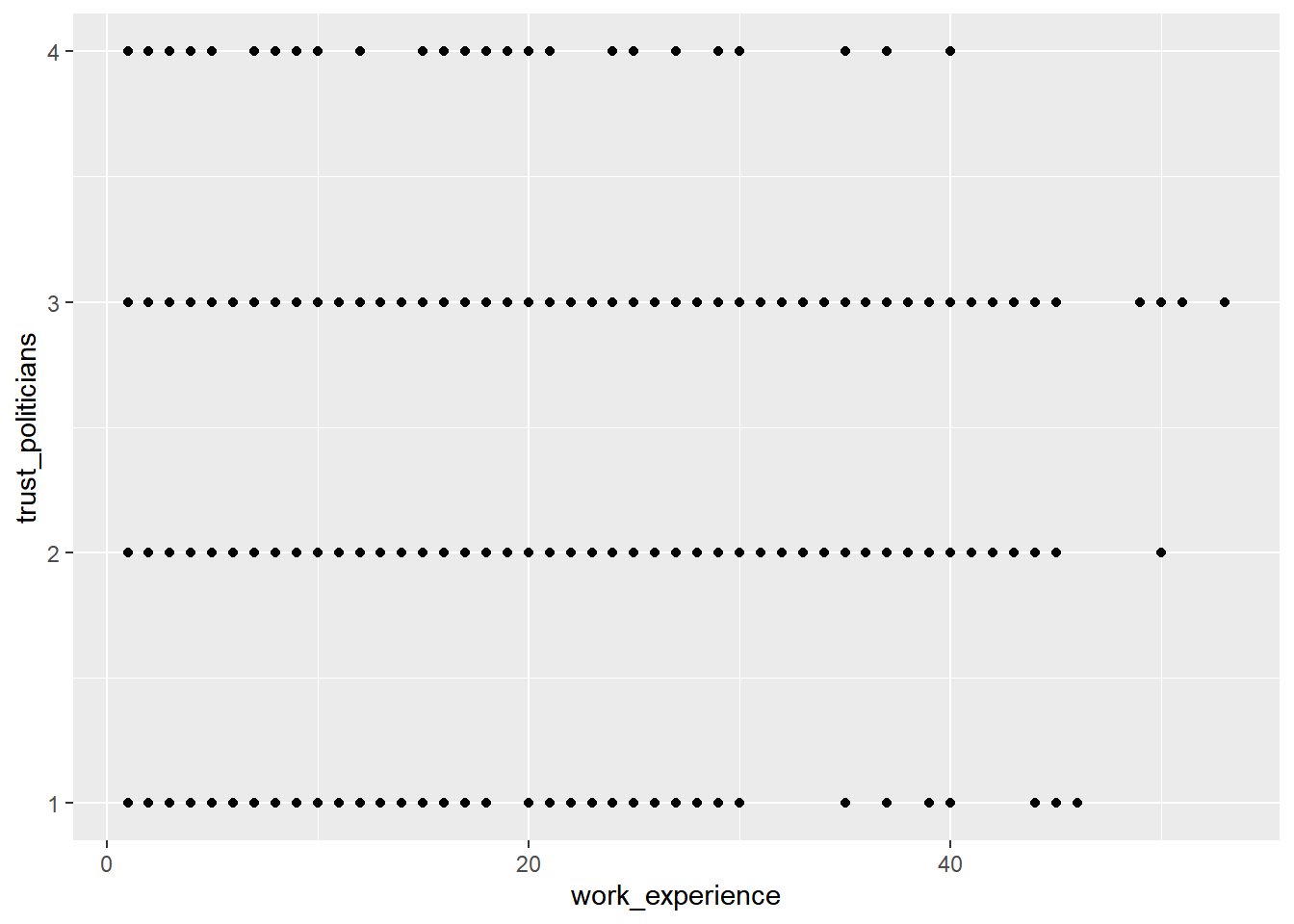
Show how journalists’ work experience (work_experience) is associated
with their trust in politicians (trust_politicians). To do this,
create a very basic scatter plot using ggplot2 and the respective
ggplot() function. Use the aes() function inside ggplot() to map
variables to the visual properties. Use geom_point() to add points to
the plot.
Solution:
Task 2
Do more experienced journalists become less trusting in politicians? Add
this code to your plot to create a regression line:
+ geom_smooth(method = lm, se = FALSE).
What can you conclude from the regression line?
Solution:
WoJ %>% ggplot(aes(x = work_experience, y = trust_politicians)) +
geom_point() +
geom_smooth(method = lm, se = FALSE)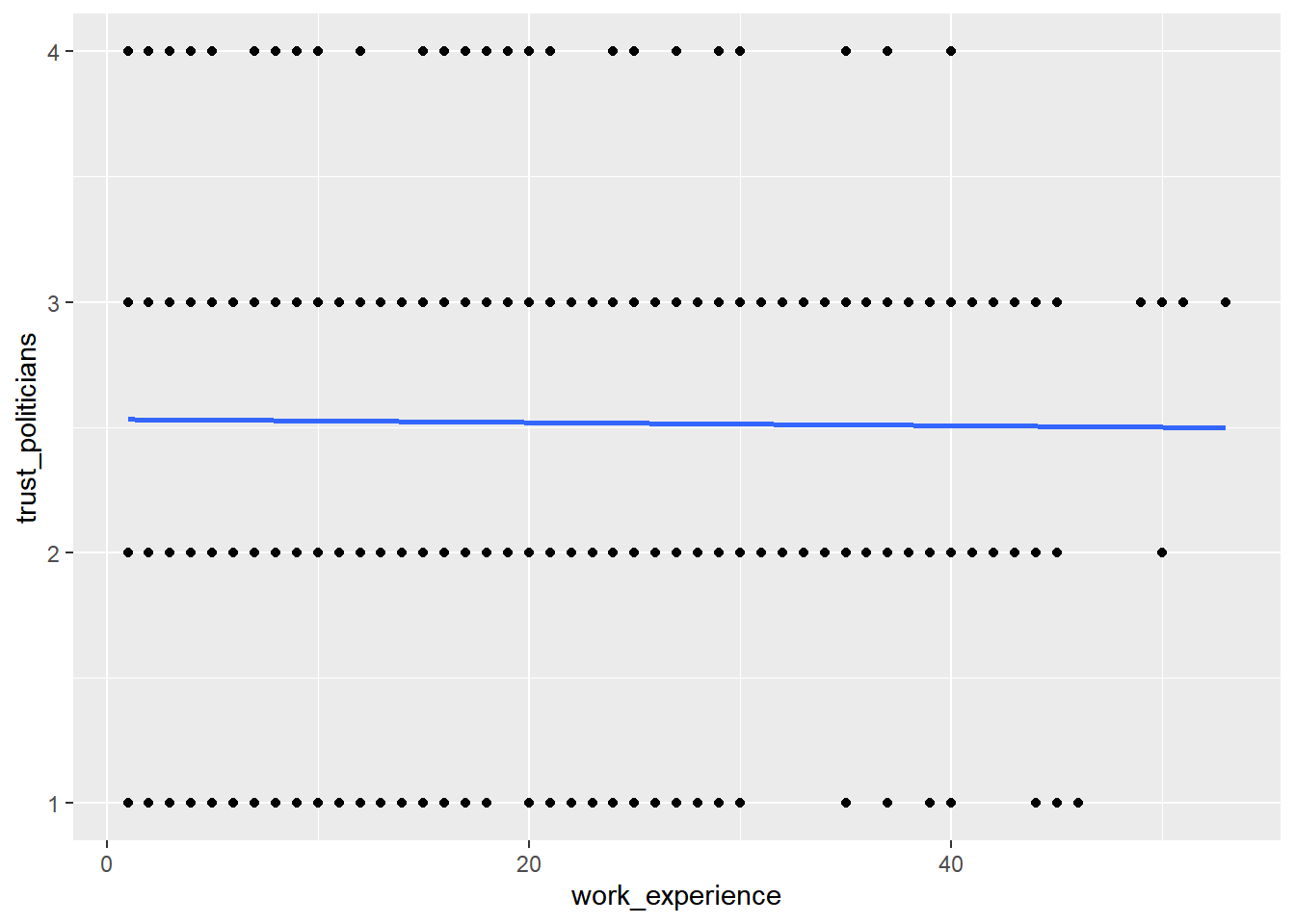
The regression line shows us that there is no relationship between work experience and trust in politicians. In other words, more experienced journalists do not become less trusting in politicians.
Task 3
Does the relationship between work experience and trust in politicians remain stable across different countries? Alternatively, does work experience influence trust in politicians differently depending on the specific country context?
Try to create a visualization to answer this question using
facet_wrap().
Solution:
WoJ %>% ggplot(aes(x = work_experience, y = trust_politicians)) +
  geom_point() +
geom_smooth(method = lm, se = FALSE) +
facet_wrap(~country)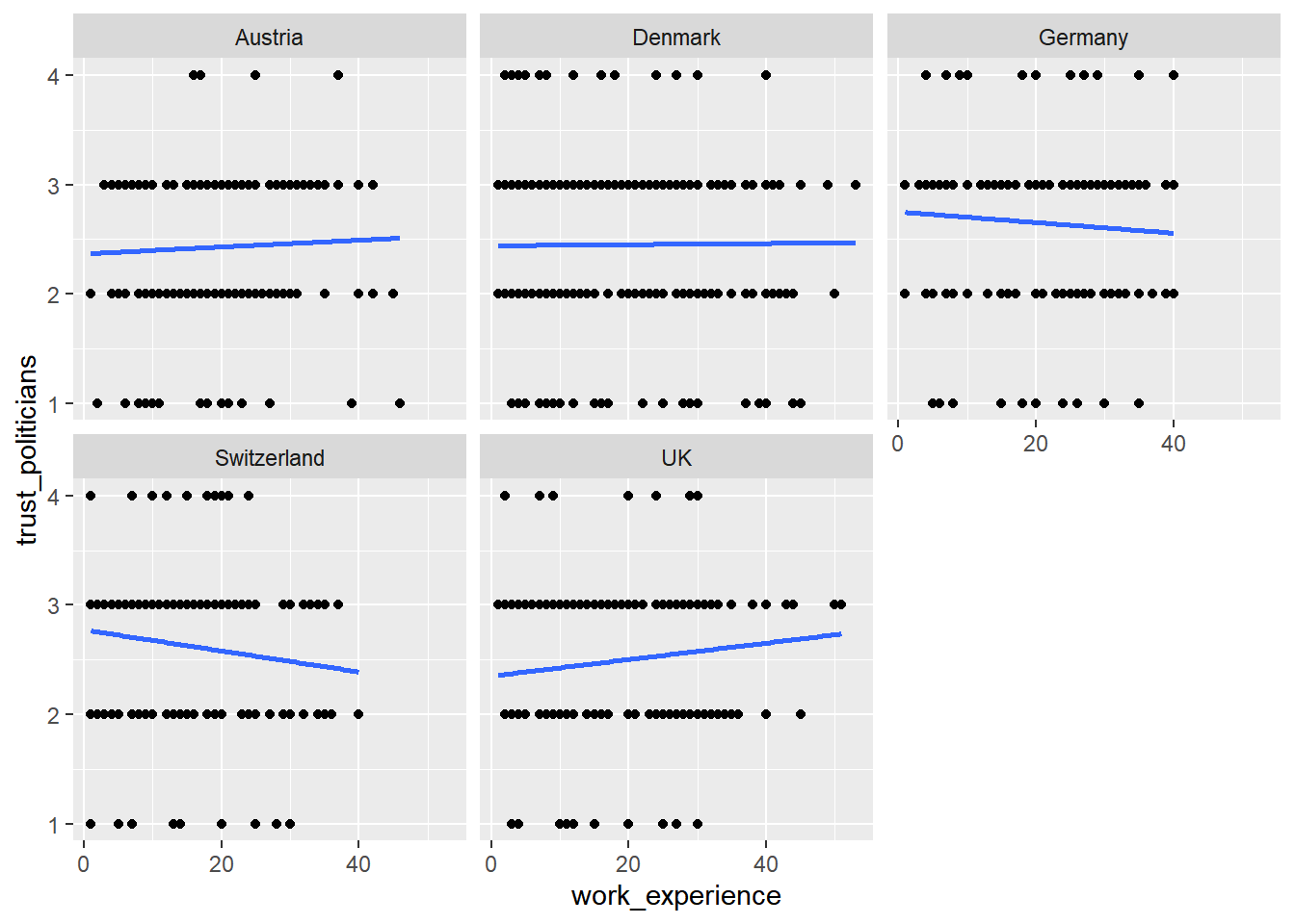
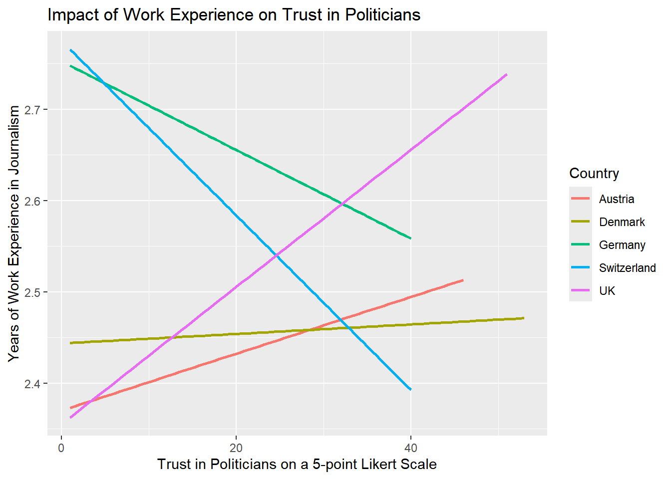
Task 4
In your current visualization, it may be challenging to discern cross-country differences. Let’s aim to create a visualization that illustrates these differences across countries more distinctly.
Remove the facet_wrap() and the geom_point() code line. This leaves
you with this graph:
WoJ %>% ggplot(aes(x = work_experience, y = trust_politicians)) +
  geom_smooth(method = lm, se = FALSE)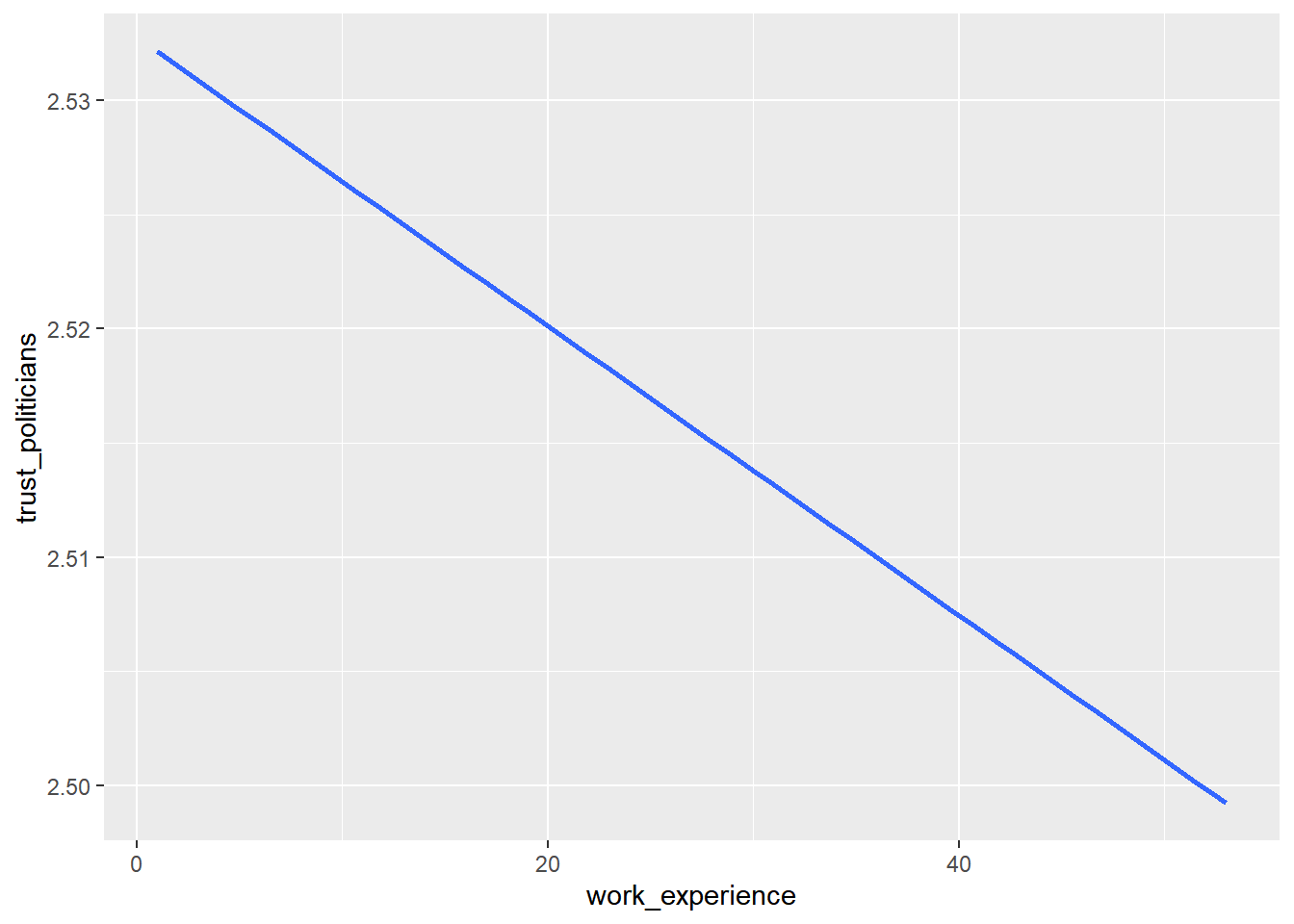
Now, display every country in a separate color by using the color
argument inside the aes() function.
Solution:
WoJ %>% ggplot(aes(x = work_experience, y = trust_politicians, color = country)) +
  geom_smooth(method = lm, se = FALSE)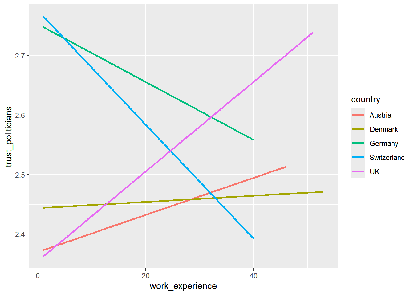
Task 5
Add fitting labels to your plot. For example, set the main title to display: “Impact of Work Experience on Trust in Politicians”. The x-axis label should read “Years of Work Experience in Journalism”, and the y-axis label should read “Trust in Politicians on a 5-point Likert Scale”. The label for the color legend should be “Country”.
Solution:
WoJ %>% ggplot(aes(x = work_experience, y = trust_politicians, color = country)) +
  geom_smooth(method = lm, se = FALSE) +
  labs(
    title = "Impact of Work Experience on Trust in Politicians",
    x = "Trust in Politicians on a 5-point Likert Scale",
    y = "Years of Work Experience in Journalism",
    color = "Country"
  )
Task 6
Add a nice theme that you like, e.g. theme_minimal(),
theme_classic() or theme_bw().
Solution:
WoJ %>% ggplot(aes(x = work_experience, y = trust_politicians, color = country)) +
  geom_smooth(method = lm, se = FALSE) +
  labs(
    title = "Impact of Work Experience on Trust in Politicians",
    x = "Trust in Politicians on a 5-point Likert Scale",
    y = "Years of Work Experience",
    color = "Country"
  ) +
  theme_bw()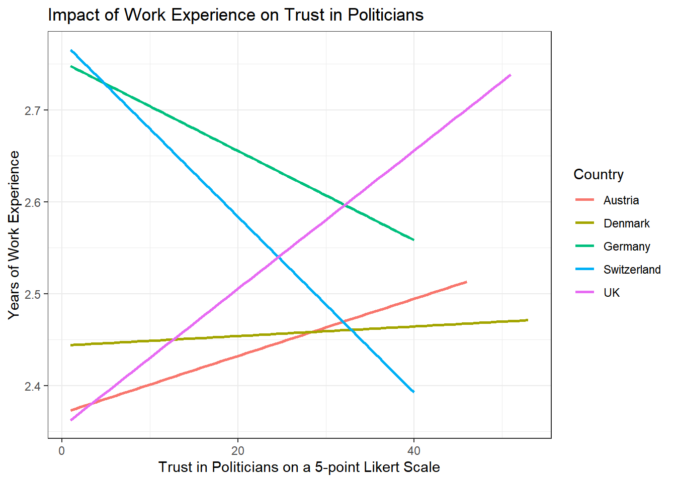
Solutions for Exercise 5
Task 1
Solution:
data %>% ggplot(aes(x = country, y = work_experience)) +
  geom_boxplot() +
  theme_bw() +
  labs(x = "Country", y = "Work Experience (Years)", title = "Distribution of Work Experience by Country")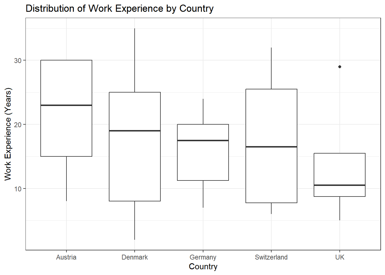
Task 2
Solution:
data %>%
  ggplot(aes(x = work_experience, y = trust_government, color = country)) +
  geom_point() +
  theme_bw() +
  labs(x = "Work Experience (Years)", y = "Trust in Government", color = "Country", title = "Trust in Government by Work Experience and Country")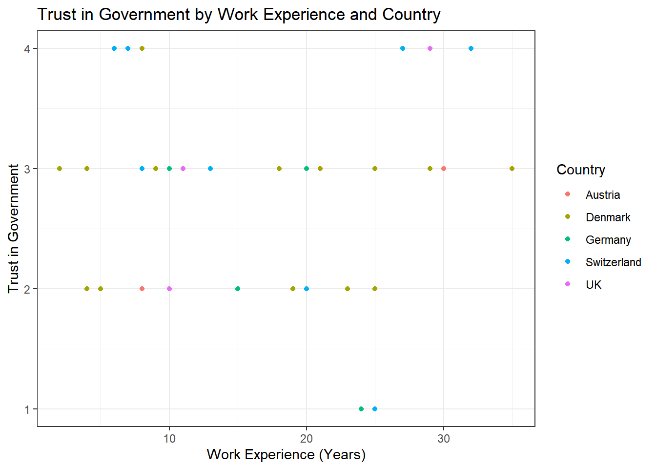
Task 3
Solution:
data %>%
  ggplot(aes(x = work_experience, y = trust_government, color = country)) +
  geom_point() +
  geom_text(aes(label = name), check_overlap = TRUE, hjust = 0, vjust = 0) +
  theme_bw() +
  labs(x = "Work Experience (Years)", y = "Trust in Government", color = "Country", title = "Trust in Government by Work Experience and Country")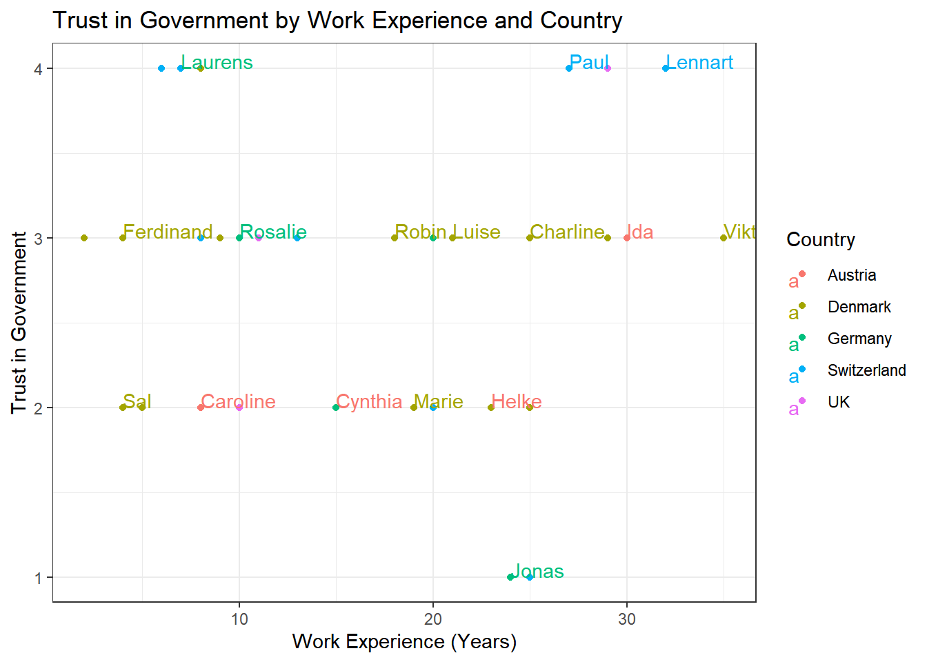
Task 4
Solution:
data %>%
  ggplot(aes(x = country, fill = employment)) +
  geom_bar(position = "dodge") +
  theme_bw() +
  labs(x = "Country", y = "Count", fill = "Employment Type", title = "Employment Types by Country")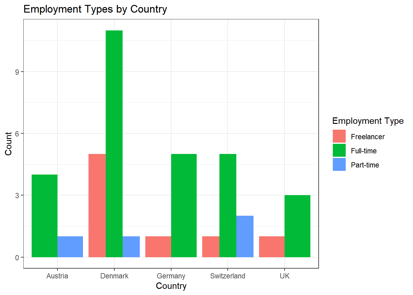
Alternative Solution: Those who prefer the width of the bars to be aligned can use this code:
data %>%
  ggplot(aes(x = country, fill = employment)) +
  geom_bar(position = position_dodge(preserve = "single")) +
  theme_bw() +
  labs(x = "Country", y = "Count", fill = "Employment Type", title = "Employment Types by Country")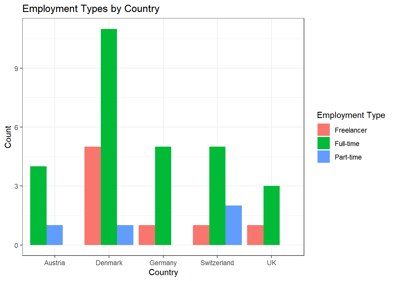
Task 5
You can solve this exercise using two approaches. The first approach is to create a new variable called experience_level and save it in your original data set to be used for data visualization in the next, separate step:
Solution:
data <- data %>%
  mutate(experience_level = case_when(
    work_experience <= 10 ~ "Junior",
    work_experience > 10 & work_experience <= 20 ~ "Mid-Level",
    work_experience > 20 ~ "Senior"
  ))

data %>%
  ggplot(aes(x = country, fill = employment)) +
  geom_bar(position = "dodge") +
  theme_bw() +
  labs(x = "Country", y = "Count", fill = "Employment Type", title = "Employment Types by Country and Level of Experience") +
  facet_wrap(~experience_level) +
  theme(axis.text.x = element_text(angle = 45, hjust = 1))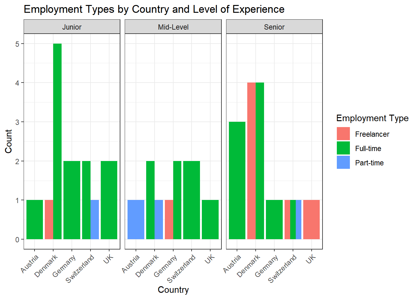
The more elegant solution is to perform your data management in one go without saving the variable experience_level back into your original data set. Using this approach will help declutter your data because you won’t need to create and save a new variable that is only required for a single visualization:
data %>%
  mutate(experience_level = case_when(
    work_experience <= 10 ~ "Junior",
    work_experience > 10 & work_experience <= 20 ~ "Mid-Level",
    work_experience > 20 ~ "Senior"
  )) %>%
  ggplot(aes(x = country, fill = employment)) +
  geom_bar(position = "dodge") +
  theme_bw() +
  labs(x = "Country", y = "Count", fill = "Employment Type", title = "Employment Types by Country and Level of Experience") +
  facet_wrap(~experience_level) +
  theme(axis.text.x = element_text(angle = 45, hjust = 1))
Solutions for Exercise 6
In this exercise, we will work with the mtcars data that comes pre-installed with dplyr.
library(tidyverse)
data <- as_tibble(mtcars)

# To make the data somewhat more interesting, let's set a few values to missing values:
data <- data %>%
  mutate(wt = na_if(wt, 4.070))

data <- data %>%
  mutate(mpg = na_if(mpg, 22.8))
Task 1
Check the data set for missing values (NAs) and delete all observations that have missing values.
Solution:
You can solve this by excluding NAs in every single column:
data <- data %>%
  # we'll now only keep observations that are NOT NAs in the following variables (remember that & = AND):
  filter(!is.na(mpg) & !is.na(cyl) & !is.na(disp) & !is.na(hp) & !is.na(drat) & !is.na(wt) & !is.na(qsec) & !is.na(vs) & !is.na(am) & !is.na(gear) & !is.na(carb))
Alternatively, excluding NAs from the entire data set works, too, but
you have not learned the drop_na()function in the tutorials:
Task 2
Let’s transform the weight wt of the cars. Currently, it’s given as Weight in 1000 lbs. I guess you are not used to lbs, so try to mutate wt to represent Weight in 1000 kg. 1000 lbs = 453.59 kg, so we will need to divide by 2.20.
Similarly, I think that you are not very familiar with the unit Miles per gallon of the mpg variable. Let’s transform it into Kilometer per liter. 1 m/g = 0.425144 km/l, so again divide by 2.20.
Solution:
Task 3
Now we want to group the weight of the cars in three categories: light, medium, heavy. But how to define light, medium, and heavy cars, i.e., at what kg should you put the threshold? A reasonable approach is to use quantiles (see Tutorial: summarize() [+ group_by()]). Quantiles divide data. For example, the 75% quantile states that exactly 75% of the data values are equal or below the quantile value. The rest of the values are equal or above it.
Use the lower quantile (0.25) and the upper quantile (0.75) to estimate two values that divide the weight of the cars in three groups. What are these values?
Solution:
You can use dplyrfor this job:
## # A tibble: 1 × 2
##   LQ_wt UQ_wt
##   <dbl> <dbl>
## 1  1.19  1.62
Or you can use the tidycomm package:
## # A tibble: 1 × 3
##   Variable   p25   p75
## * <chr>    <dbl> <dbl>
## 1 wt        1.19  1.62
75% of all cars weigh 1.622727* 1000kg or less and 25% of all cars weigh 1.190909* 1000kg or less.
Task 4
Use the values from Task 3 to create a new variable wt_cat that divides the cars in three groups: light, medium, and heavy cars.
Solution:
You can use dplyr:
data <- data %>%
  mutate(wt_cat = case_when(
    wt <= 1.190909 ~ "light car",
    wt < 1.622727 ~ "medium car",
    wt >= 1.622727 ~ "heavy car"
  ))
Or tidycomm:
Task 5
How many light, medium, and heavy cars are part of the data?
Solution:
You can solve this with the summarize(count = n() function:
## # A tibble: 3 × 2
##   wt_cat     count
##   <chr>      <int>
## 1 heavy car      9
## 2 light car      7
## 3 medium car    13
9 heavy cars, 13 medium cars, and 7 light cars.
Alternatively, you can also use the count() function:
## # A tibble: 3 × 2
##   wt_cat         n
##   <chr>      <int>
## 1 heavy car      9
## 2 light car      7
## 3 medium car    13
Alternatively, you can use the tab_frequencies() fucntion of the
tidycomm:
## # A tibble: 3 × 5
##   wt_cat         n percent cum_n cum_percent
## * <chr>      <int>   <dbl> <int>       <dbl>
## 1 heavy car      9   0.310     9       0.310
## 2 light car      7   0.241    16       0.552
## 3 medium car    13   0.448    29       1
Task 6
Now sort this count of the car weight classes from highest to lowest.
Solution:
## # A tibble: 3 × 2
##   wt_cat     count
##   <chr>      <int>
## 1 medium car    13
## 2 heavy car      9
## 3 light car      7
Alternatively, use tidycomm:
## # A tibble: 3 × 5
##   wt_cat         n percent cum_n cum_percent
##   <chr>      <int>   <dbl> <int>       <dbl>
## 1 medium car    13   0.448    29       1
## 2 heavy car      9   0.310     9       0.310
## 3 light car      7   0.241    16       0.552
Task 7
Make a scatter plot to indicate how many km per liter (mpg) a car can drive depending on its weight (wt). Facet the plot by weight class (wt_cat).
Solution:
data %>%
  mutate(wt_cat = factor(wt_cat, levels = c("light car", "medium car", "heavy car"))) %>%
  ggplot(aes(x = wt, y = mpg)) +
  geom_point() +
  theme_bw() +
  labs(title = "Relationship between car weight and achieved kilometers per liter", x = "Weight in 1000kg", y = "km/l") +
  facet_wrap(~wt_cat)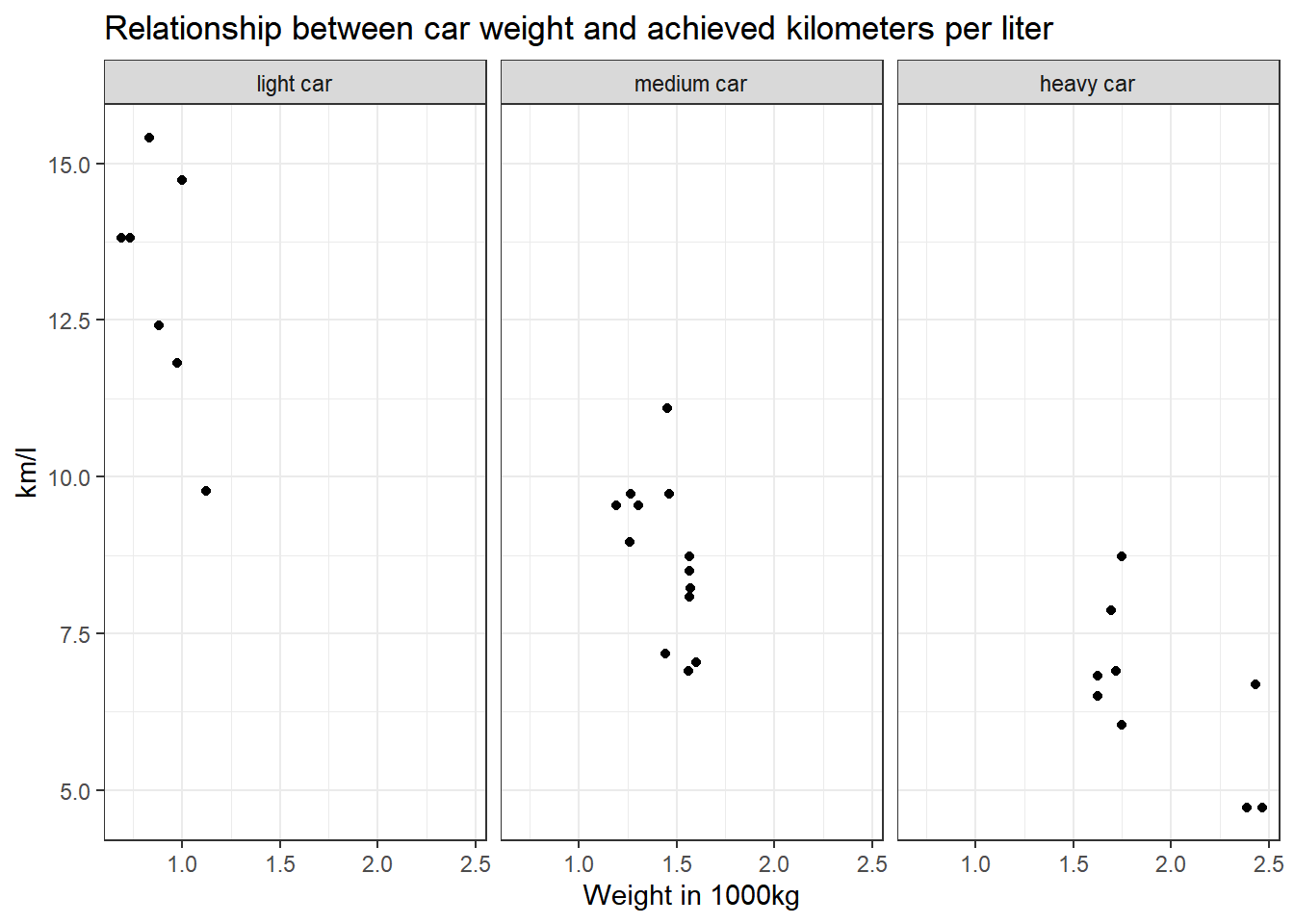
Alternatively, you can use tidycomm:
data %>%
  mutate(wt_cat = factor(wt_cat, levels = c("light car", "medium car", "heavy car"))) %>%
  tidycomm::correlate(wt, mpg) %>%
  tidycomm::visualize() +
  labs(title = "Relationship between car weight and\n achieved kilometers per liter", x = "Weight in 1000kg", y = "km/l") +
  theme_bw() +
  facet_wrap(~wt_cat)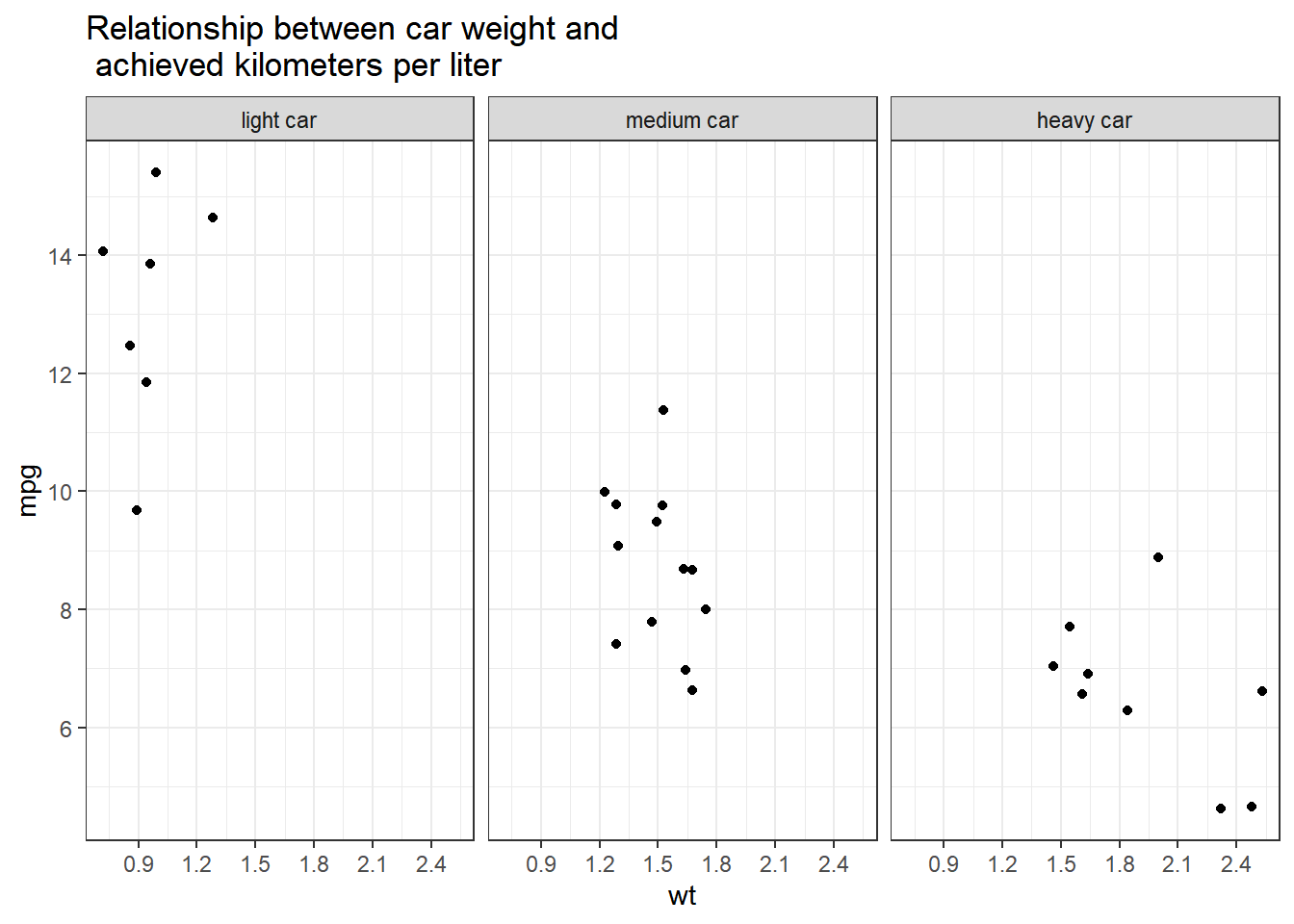
Task 8
Recreate the diagram from Task 7, but exclude all cars that weigh between 1.4613636 and 1.5636364 *1000kg from it.
Solution:
data %>%
  filter(wt < 1.4613636 | wt > 1.5636364) %>%
  mutate(wt_cat = factor(wt_cat, levels = c("light car", "medium car", "heavy car"))) %>%
  ggplot(aes(x = wt, y = mpg)) +
  geom_point() +
  theme_bw() +
  theme(legend.position = "none") +
  labs(title = "Relationship between car weight and achieved kilometers per liter", x = "Weight in 1000kg", y = "km/l") +
  facet_wrap(~wt_cat)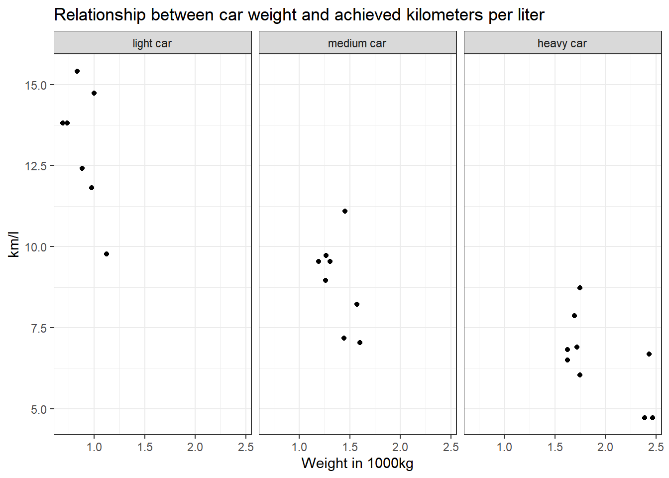
With tidycomm:
data %>%
  filter(wt < 1.4613636 | wt > 1.5636364) %>%
  mutate(wt_cat = factor(wt_cat, levels = c("light car", "medium car", "heavy car"))) %>%
  tidycomm::correlate(wt, mpg) %>%
  tidycomm::visualize() +
  labs(title = "Relationship between car weight and achieved kilometers per liter", x = "Weight in 1000kg", y = "km/l") +
  theme_bw() +
  facet_wrap(~wt_cat)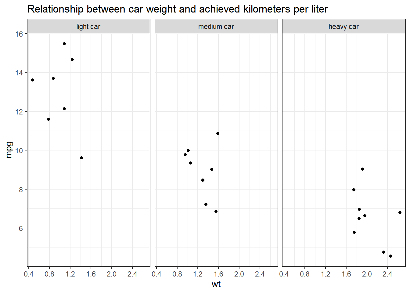
Why would we use data %>% filter(wt < 1.4613636 | wt > 1.5636364)
instead of data %>% filter(wt > 1.4613636 | wt < 1.5636364)?
Let’s look at the resulting data sets when you apply those filters to compare them:
## # A tibble: 24 × 1
##       wt
##    <dbl>
##  1  1.19
##  2  1.31
##  3  1.57
##  4  1.62
##  5  1.45
##  6  1.70
##  7  1.72
##  8  2.39
##  9  2.47
## 10  2.43
## # ℹ 14 more rows
The resulting table does not include any cars that weigh between
1.4613636 and 1.5636364. But if you use
data %>% filter(wt > 1.4613636 | wt < 1.5636364)…
## # A tibble: 29 × 1
##       wt
##    <dbl>
##  1  1.19
##  2  1.31
##  3  1.46
##  4  1.56
##  5  1.57
##  6  1.62
##  7  1.45
##  8  1.56
##  9  1.56
## 10  1.70
## # ℹ 19 more rows
… cars that weigh between 1.4613636 and 1.5636364 are still included!
But why? The filter()function always keeps cases based on the
criteria that you provide.
In plain English, my solution code says the following: Take my dataset “data” and keep only those cases where the weight variable wt is less than 1.4613636 OR larger than 1.5636364. Put differently, the solution code says: Delete all cases that are greater than 1.4613636 but are also less than 1.5636364.
The wrong code, on the other hand, says: Take my dataset “data” and keep only those cases where the weight variable wt is greater than 1.4613636 OR smaller than 1.5636364. This is ALL the data because all your cases will be greater than 1.4613636 OR smaller than 1.5636364. You are not excluding any cars.