8 Tidy text analysis

After working through Tutorial 7, you’ll…

• understand the concept of tidy text
• know how to combine tidy text management approaches with regular expressions
• be able to produce first analyses, e.g., word frequencies

8.1 What is tidy text?

Since you’ve already learnt what tidy data is (see Tidy data), you can make an educated guess about the meaning of “tidy text”! In contrast to the ways text is commonly stored in existing text analysis approaches (e.g., as strings or document-term matrices), the tidy text format is a table with one single token per row (token = the unit of analysis). A token is a meaningful unit of text, i.e., a word, a sentence, or a paragraph that we are interested in using for further analysis. Splitting text into tokens is what we call the process of tokenization.

Julia Silge and David Robinson’s tidytext package makes tokenizing into the tidy text format simple! Moreover, the tidytext package builds upon tidyverse and ggplot2, which makes it easy to use for you, since you already know these packages (see Tutorial: Data management with tidyverse and Tutorial: Data visualization with ggplot for a recap). That’s why we’ll focus on the tidytext in this session.

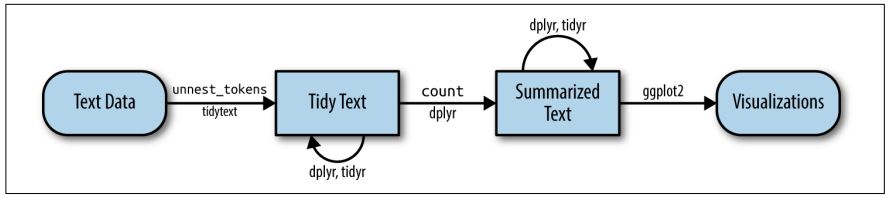
This tutorial is based on Julia Silge and David Robinson’s open-access book “Text Mining in R. A Tidy Approach” and a lot of the following code was actually written by Julia Silge. If you want to dig deeper into tidy text analysis, you should check the book out. Both authors have also created an informative flowchart of the tidy text analysis workflow:

Image: Tidy Text Analysis Workflow

Before we start, install and load the tidytext package and the tidyverse package.

# installing/loading the package:
if(!require(tidytext)) {
  install.packages("tidytext"); 
  require(tidytext)
} #load / install+load tidytext

# installing/loading tidyverse:
if(!require(tidyverse)) {
  install.packages("tidyverse"); 
  require(tidyverse)
} #load / install+load tidyverse

8.2 Preprocessing real-world data

Let’s investigate what the tidytext package is capable of and apply it to some real-world data. I’ve provided you with a data file that contains data collected with the Twitter API about the Russian aggression against Ukraine on Moodle.

Let’s import the data into RStudio and inspect it using the View() function.

data <- read.csv("ukraine_tweets.csv", encoding = "UTF-8") # Use UTF-8 encoding to keep the smileys

View(data)

The date column is a character variable. Let’s convert the date column to a standard format using the lubridate package of the tidyverse, making it easier to create graphs using time data later on.

data <- data %>% 
  mutate(time = lubridate::ymd_hms(time)) %>%  # turn the data column into a proper format with the lubridate package (this helps to create time series graphs!)
  tibble()

View(data)

This data set contains a lot of information! We get to know who wrote the tweet (user and the unique user.id) and where this person lives (user.location). But most importantly, we can find the text of the tweet in the column full_text.

First of all, let’s reduce some of these columns that we don’t need for our text analysis.

data_short <- data %>% 
  select(time, user, full_text) # keeps time, user, and full_text

View(data_short)

Now, to get an overview, let’s create a visualization of the user’s who posted at least 18 tweets.

data_short %>%
  group_by(user) %>%
  summarize(n = n()) %>%
  filter(n > 18) %>%
  ggplot(aes(x = user, y = n)) +
  stat_summary(geom = "bar") +
  theme_bw() +
  theme(axis.text.x = element_text(angle = 90, vjust = 0.00, hjust = 0.00)) +
  labs(title = "Users who posted the most tweets about the Russian\naggression against Ukraine",
       x = "User name", y = "Number of Tweets")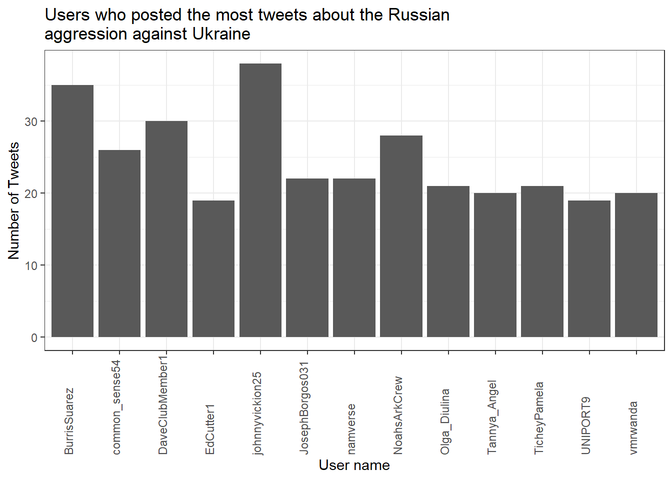

Now that we have had our overview, we will start with a process called text normalization. Text normalization is the endeavor to minimize the variability of a text by bringing it closer to a specified “standard” by reducing the quantity of divergent data that the computer has to deal with. In plain English, this means that our goal is to reduce the amount of text to a small set of words that are especially suitable to explain similarities and differences between tweets and, more interestingly, between the accounts that have published these tweets. Overall, text normalization boosts efficiency. Some techniques of text normalization will be covered in the next few sections, for example, tokenization, stop word removal, stemming/lemmatization and pruning. You could add additional steps, e.g. spelling corrections to reduce misspellings that increase word variance, but we won’t cover all text normalization steps in this tutorial.

8.2.1 Tokenization

I think we are ready to tokenize the data with the amazing unnest_tokens() function of the tidytext package. Tokenization is the process of breaking text into words (and punctuation marks). Since scientists are almost never interested in the punctuation marks and will delete them from the data set later anyway, unnest_tokens() comes with the nice bonus of setting all text to lowercase and deleting the punctuation marks directly, leaving only words (and numbers) as tokens.

A common practice is to remove all tokens that contain numbers. Depending on the research question, it can also be helpful to remove URLs. For illustrative purposes, we will do both. But keep in mind that removing all URLs will take the option from you to compare what accounts have shared certain URLs more frequently than others.

remove_reg <- "&amp;|&lt;|&gt;" # &amp; = & in HTML,  &lt; = < in HTML,   &gt; = > in HTML

data_tknzd <- data_short %>%
  mutate(tweet = row_number()) %>% # creates a new column that is called "tweet", which contains a unique id for each individual tweet based on its row number
  filter(!str_detect(full_text, "^RT")) %>%  # removes all retweets, i.e., tweets that are not unique but a reposts
  mutate(text = str_remove_all(full_text, remove_reg)) %>%  # remove special HTML characters (&, <, >)
  unnest_tokens(word, full_text) %>%
  filter(!str_detect(word, "^[:digit:]+$")) %>%             # remove all words that are numbers, e.g. "2020"
  filter(!str_detect(word, "^http")) %>%                    # remove all words that are a URL, e.g., (https://evoldyn.gitlab.io/evomics-2018/ref-sheets/R_strings.pdf)
  filter(!str_detect(word, "^(\\+)+$")) %>%                 #  remove all words that only consist of plus signs (e.g., "+++")
  filter(!str_detect(word, "^(\\+)+(.)+$")) %>%             #  remove all words that only consist of plus signs followed by any other characters (e.g., "+++eil+++")
  filter(!str_detect(word, "^(\\-)+$")) %>%                 #  remove all words that only consist of plus signs (e.g., "---")
  filter(!str_detect(word, "^(\\-)+(.)+$")) %>%             #  remove all words that only consist of minus signs followed by any other characters (e.g., "---eil---")
  filter(!str_detect(word, "^(.)+(\\+)+$"))                 # remove all words that start with some kind of word followed by plus signs (e.g., "news+++")

head(data_tknzd)

## # A tibble: 6 × 5
##   time                user     tweet text                                  word 
##   <dttm>              <chr>    <int> <chr>                                 <chr>
## 1 2022-02-25 18:10:59 peekay14     1 @vonderleyen @EU_Commission rubbish!… vond…
## 2 2022-02-25 18:10:59 peekay14     1 @vonderleyen @EU_Commission rubbish!… eu_c…
## 3 2022-02-25 18:10:59 peekay14     1 @vonderleyen @EU_Commission rubbish!… rubb…
## 4 2022-02-25 18:10:59 peekay14     1 @vonderleyen @EU_Commission rubbish!… your 
## 5 2022-02-25 18:10:59 peekay14     1 @vonderleyen @EU_Commission rubbish!… words
## 6 2022-02-25 18:10:59 peekay14     1 @vonderleyen @EU_Commission rubbish!… and

Now, let’s check the total number of unique words in our tweet data:

paste("We are investigating ", dim(data_tknzd)[1], " non-unique features / words and ", length(unique(data_tknzd$word)), " unique features / words.")

## [1] "We are investigating  259873  non-unique features / words and  25922  unique features / words."

Remember: unnest tokens() comes with a few handy preprocessing features, i.e., it already turns the text into a standardized format for further analysis:

1. Tweet ids from which each word originated are kept in the data frame (column: tweet).
2. All punctuation has already been taken care of, i.e., dots, questions marks, etc. have been removed.
3. All uppercase letters have been taken care of, i.e., words have been transformed to lowercase.⁴

Practice: Tokenization

Now it’s your turn. I’ve added another data set to Moodle that deals with the shitstorm about the German influencer Fynn Kliemann on Twitter. You can read more about the scandal that started on the 6th of May 2022 here if you feel that you need more information.

Load the Kliemann data into RStudio. Use the tutorial code and to set the encoding and to convert the date column to a standardized date format. After loading the Kliemann data keep only the time, user, and full_text column.

Next, try to tokenize the data.

For solutions see: Solutions for Exercise 6

8.2.2 Stop word removal

Next, we should get rid of stop words. Stop words are a group of words that are regularly used in a language. In English, stop words such as “the,” “is,” and “and” would qualify. Because stop words are so common, they don’t really tell us anything about the content of a tweet and what differentiates this tweet from other tweets. The tidytext package comes with a pre-installed stop word data set. Let’s save that data set to a source object called stop_word_data. This way, we can use it later.

stop_word_data <- tidytext::stop_words

head(stop_word_data, 20) # prints the first 20 stop words to the console

## # A tibble: 20 × 2
##    word        lexicon
##    <chr>       <chr>  
##  1 a           SMART  
##  2 a's         SMART  
##  3 able        SMART  
##  4 about       SMART  
##  5 above       SMART  
##  6 according   SMART  
##  7 accordingly SMART  
##  8 across      SMART  
##  9 actually    SMART  
## 10 after       SMART  
## 11 afterwards  SMART  
## 12 again       SMART  
## 13 against     SMART  
## 14 ain't       SMART  
## 15 all         SMART  
## 16 allow       SMART  
## 17 allows      SMART  
## 18 almost      SMART  
## 19 alone       SMART  
## 20 along       SMART

Now, let’s use these stop words to remove all tokens that are stop words from our tweet data.

data_tknzd <- data_tknzd %>% 
  filter(!word %in% stop_word_data$word) %>%  # removes all of our tokens that are stop words
  filter(!word %in% str_remove_all(stop_word_data$word, "'")) # first removes all ' from the stop words (e.g., ain't -> aint) and then removes all of our tokens that resemble these stop words without punctuation

Practice: Stop word removal

Now it’s your turn. The Kliemann data is in German, so you can’t use the tidytext stop word list, which is meant for English text only. So install and load the ‘stopwords’ package that allows you to create a dataframe that contains German stop words by using this command: stop_word_german <- data.frame(word = stopwords::stopwords("de"), stringsAsFactors = FALSE). Create your German stop word list and use it to remove stop words from your tokens.

For solutions see: Solutions for Exercise 6

8.2.3 Lemmatizing & stemming

Minimizing words to their basic form (lemmatizing) or root (stemming) is a typical strategy of reducing the number of words in a text.

1. Stemming: A stem is the root form of a word without any suffixes. A stemming algorithm (= stemmer) removes the suffixes and returns the stem of the word. Example1: vengeance –> vengeanc, or, if you use a very aggressive stemmer, vengeance –> veng || Example2: legions –> legion, or, if you use a very aggressive stemmer, legions –> leg (this one is problematic!) || Example3: murdered –> murder

2. Lemmatization: A lemma is a lexicon headword or, i.e., the dictionary-matched basic form of a word (as opposed to a stem created by eliminating or changing suffixes). Because a lemmatizing algorithm (= lemmatizer) performs dictionary matching, lemmatization is more computationally demanding than stemming. vengeance –> vengeance || Example2: legions –> legion || Example3: murdered –> murdered (this one is problematic!)

Most of the time, stemmers will make a lot of mistakes (e.g., legions –> leg) and lemmatizers will make fewer mistakes. However, lemmatizers summarize fewer words (murdered –> murdered) and therefore reduce the word count less efficiently than stemmers. Which technique of text normalization is preferred is always determined by the research question and the available data.

For the ease of teaching, we will use stemming on our tweet data. However, you could also use lemmatization with the spacyr package.

We’ll use Porter’s (1980) stemming algorthm, which is the most extensively used stemmer for the English language. Porter made the stemmer open-source, and you may use it with R using the SnowballC package (Bouchet-Valat 2020).

# installing/loading SnowballC:
if(!require(SnowballC)) {
  install.packages("SnowballC"); 
  require(SnowballC)
} #load / install+load SnowballC

data_tknzd <- data_tknzd %>%
  mutate(word = wordStem(word))

head(data_tknzd)

## # A tibble: 6 × 5
##   time                user     tweet text                                  word 
##   <dttm>              <chr>    <int> <chr>                                 <chr>
## 1 2022-02-25 18:10:59 peekay14     1 @vonderleyen @EU_Commission rubbish!… vond…
## 2 2022-02-25 18:10:59 peekay14     1 @vonderleyen @EU_Commission rubbish!… eu_c…
## 3 2022-02-25 18:10:59 peekay14     1 @vonderleyen @EU_Commission rubbish!… rubb…
## 4 2022-02-25 18:10:59 peekay14     1 @vonderleyen @EU_Commission rubbish!… word 
## 5 2022-02-25 18:10:59 peekay14     1 @vonderleyen @EU_Commission rubbish!… fell…
## 6 2022-02-25 18:10:59 peekay14     1 @vonderleyen @EU_Commission rubbish!… eu

Let’s check how many unique words we have in our tweet data after all of our preprocessing efforts:

paste("We are investigating ", dim(data_tknzd)[1], " non-unique features / words and ", length(unique(data_tknzd$word)), " unique features / words.")

## [1] "We are investigating  130045  non-unique features / words and  21188  unique features / words."

Practice: Lemmatizing & stemming

Please stem the Kliemann data with the PorterStemmer. Since we are working with German data, you’ll have to add the option language = "german" to the wordStem() function.

For solutions see: Solutions for Exercise 6

8.2.4 Pruning

Finally, words that appear in practically every tweet (i.e., promiscuous words) or words that that appear only once or twice in the entire data set (i.e., rare words) are not very helpful for investigating the “typical” word use of certain Twitter accounts. Since these words do not contribute to capturing similarities and differences in texts, it is a good idea to remove them. This process of (relative) pruning is quickly achieved with the quanteda package. Since I don’t want to teach you how to use quanteda just yet, I have developed a useful short cut function that enables you to use relative pruning without having to learn quanteda functions.

First, install/load the quanteda package and initialize my prune-function by running this code:

# Install / load the quanteda package
if(!require(quanteda)) {
  install.packages("quanteda"); 
  require(quanteda)
} #load / install+load quanteda

prune <- function(data, tweet_column, word_column, text_column, user_column, minDocFreq, maxDocFreq) {
suppressWarnings(suppressMessages(library("quanteda", quietly = T)))
# Grab the variable names for later use
tweet_name <- substitute(tweet_column)
word_name <- substitute(word_column)
tweet_name_chr <- as.character(substitute(tweet_column))
word_name_chr <- as.character(substitute(word_column))
# turn the tidy data frame into a document-feature matrix:
dfm <- data %>%
  select({{tweet_column}}, {{text_column}}, {{word_column}}, {{user_column}}) %>%
  count({{tweet_column}}, {{word_column}}, sort = TRUE) %>% 
  cast_dfm({{tweet_column}}, {{word_column}}, n)
# perform relative pruning:
dfm <- dfm_trim(dfm, 
                min_docfreq = minDocFreq, # remove all words that occur in less than minDocFreq% of all tweets
                max_docfreq = maxDocFreq, # remove all words that occur in more than maxDocFreq% of all tweets
                docfreq_type = "prop",    # use probabilities
                verbose = FALSE)          # don't tell us what you have achieved with relative pruning
# turn the document-feature-matrix back into a tidy data frame:
data2 <- tidy(dfm) %>% 
  rename({{word_name}} := term) %>% # rename columns so that their names from data_tknzd and data_tknzd2 match
  rename({{tweet_name}} := document) %>%
  select(-count) %>% # remove the count column
  mutate({{tweet_name}} :=  as.integer({{tweet_name}}))

# delete the words that quanteda suggested from the original data
data <- right_join(data, data2, by = c(word_name_chr,tweet_name_chr)) %>% # keep only the shorter data set without frequent/rare words, but fill in all other columns like user and date
  distinct({{tweet_name}},{{word_name}}, .keep_all= TRUE) # remove duplicate rows that have been created during the merging process
return(data)
}

Now that you have my prune() function running, you can use it to prune your data. The prune function takes the following arguments:

1. data: the name of your data set (here: data_tknzd),
2. tweet_column: the name of the column that contains the tweet ids (here: tweet)
3. word_column: the name of the column that contains the words/tokens (here: word), the name of the column that contains the full text of the tweets (here: text)
4. text_column: the name of the column that contains the tweets’ full text (here: text)
5. user_column: the name of the column that contains the user names (here: user)
6. minDocFreq: the minimum values of a word’s occurrence in tweets, below which super rare words will be removed (e.g., occurs in less than 0.01% of all tweets, we choose here: 0.001)
7. maxDocFreq: the maximum values of a word’s occurrence in tweets, above which super promiscuous words will be removed (e.g., occurs in more than 95% of all tweets, we choose here: 0.95)

# Install / load the quanteda package for topic modeling
data_tknzd <- prune(data_tknzd,tweet,word,text,user, 0.001, 0.95)

Finally, now that we have removed very rare and very frequent words, let’s check the number of our unique words again:

paste("We are investigating ", dim(data_tknzd)[1], " non-unique features / words and ", length(unique(data_tknzd$word)), " unique features / words.")

## [1] "We are investigating  90806  non-unique features / words and  1762  unique features / words."

Great, we have finished the text normalization process! I think we are ready to take a sneak peek at our most common words! What are the 10 most commonly used words in our tweet data? I’m excited!

data_tknzd %>%
  count(word, sort = TRUE) %>%
  slice_head(n=10)

## # A tibble: 10 × 2
##    word        n
##    <chr>   <int>
##  1 ukrain   8873
##  2 t.co     4110
##  3 russia   2419
##  4 putin    1453
##  5 russian  1320
##  6 war      1136
##  7 peopl    1111
##  8 nato     1048
##  9 invas     706
## 10 countri   644

Evaluation: Shortly after Russia’s invasion of Ukraine began, Twitter conversations centered on the countries Ukraine, Russia, Putin, the people, the war, NATO, and the invasion.

Practice: Pruning

Please, try the prune function for yourself. Prune the Kliemann data and remove 1) words that occur in less than 0.03% of all tweets and 2) words that occur in more than 95% of all tweets. Beware: Pruning is a demanding task, therefore your machine might need a while to complete the computations. Wait until the red stop sign in your console vanishes.

For solutions see: Solutions for Exercise 6

8.3 Topic modeling

Now that we have finished our text normalization process, let’s get some results!

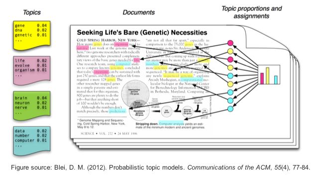
In this section, we’ll use a combination of the tidytext package and the stm package to create topic models with Latent Dirichlet allocation (LDA), one of the most prevalent topic modeling algorithms. LDA creates mixed-membership models, i.e., LDA assumes that every text contains a mix of different topics, e.g. a tweet can be 60% about TopicA (War crimes) and 40% about TopicB (Housing of refugees). Topics are defined by the mix of words that are associated with them. For example, the most common words in TopicA (War crimes) can be “massacre”, “soldiers”, and “brutal”. The most common words in TopicB (Housing of refugees) can be “volunteers”, “shelter”, and “children”. However, both topics can be mentioned in one single text, e.g., tweets about the brutal war crimes of Russian soldiers that force Ukrainian refugees to take their children and seek shelter in neighboring countries. LDA estimates the most common words in a topic and the most common topics in a text simultaneously.

Image: Assigning topics to a document (Screenshot from: Chris Bail):

Important hint: The stm package uses machine learning lingo. That is, words are called features and texts/tweets are called documents. The total sum of all documents is called a corpus. In the long run, you should get used to this lingo, so we will keep using it in this tutorial, too.

8.3.1 First steps: Create a sparse matrix

If you haven’t already, please install stm and tidytext packages:

# Install / load the stm package for topic modeling
if(!require(stm)) {
  install.packages("stm"); 
  require(stm)
} #load / install+load stm

# Install / load the tidytext package for topic modeling
if(!require(tidytext)) {
  install.packages("tidytext"); 
  require(tidytext)
} #load / install+load tidytext

First, using the tidytext package, we will convert our tidy text data into a sparse matrix that the stm package can understand for its LDA algorithm and do calculations with. For this we reshape our tokenized data into a new format called sparse matrix. In a sparse matrix…

1. …rows represent the documents (= texts),
2. …columns represent features (= unique words),
3. …the cells represent whether this word is present (1) or not present (.) in this document.

data_sparse <- data_tknzd %>%
  select(tweet, text, word) %>%
  count(tweet, word, sort = TRUE) %>% 
  cast_sparse(tweet, word, n)

head(data_sparse)

## 6 x 1762 sparse Matrix of class "dgCMatrix"
##                                                                               
## 1  1 1 1 1 1 1 1 1 1 1 1 1 1 1 1 1 1 1 1 . . . . . . . . . . . . . . . . . . .
## 11 . . . . . . . . . . . . . . . 1 . . . 1 1 1 1 . . . . . . . . . . . . . . .
## 12 . . . . . . . . . . . . . . . 1 . . . . . . . 1 1 . . . . . . . . . . . . .
## 17 . . . . . . . . . . . . . . 1 1 . . . . . . . . . 1 1 1 1 . . . . . . . . .
## 24 . . . . . . . . . . . . . . . 1 . . . . . . 1 . . . . 1 . 1 1 1 1 1 1 1 1 1
## 31 . . . . . . . . . . . . . . . 1 . . . . . 1 1 . . . . . . . . . . . . . . .
##                                                                               
## 1  . . . . . . . . . . . . . . . . . . . . . . . . . . . . . . . . . . . . . .
## 11 . . . . . . . . . . . . . . . . . . . . . . . . . . . . . . . . . . . . . .
## 12 . . . . . . . . . . . . . . . . . . . . . . . . . . . . . . . . . . . . . .
## 17 . . . . . . . . . . . . . . . . . . . . . . . . . . . . . . . . . . . . . .
## 24 1 . . . . . . . . . . . . . . . . . . . . . . . . . . . . . . . . . . . . .
## 31 . 1 1 1 1 . . . . . . . . . . . . . . . . . . . . . . . . . . . . . . . . .
##                                                                               
## 1  . . . . . . . . . . . . . . . . . . . . . . . . . . . . . . . . . . . . . .
## 11 . . . . . . . . . . . . . . . . . . . . . . . . . . . . . . . . . . . . . .
## 12 . . . . . . . . . . . . . . . . . . . . . . . . . . . . . . . . . . . . . .
## 17 . . . . . . . . . . . . . . . . . . . . . . . . . . . . . . . . . . . . . .
## 24 . . . . . . . . . . . . . . . . . . . . . . . . . . . . . . . . . . . . . .
## 31 . . . . . . . . . . . . . . . . . . . . . . . . . . . . . . . . . . . . . .
##                                                                               
## 1  . . . . . . . . . . . . . . . . . . . . . . . . . . . . . . . . . . . . . .
## 11 . . . . . . . . . . . . . . . . . . . . . . . . . . . . . . . . . . . . . .
## 12 . . . . . . . . . . . . . . . . . . . . . . . . . . . . . . . . . . . . . .
## 17 . . . . . . . . . . . . . . . . . . . . . . . . . . . . . . . . . . . . . .
## 24 . . . . . . . . . . . . . . . . . . . . . . . . . . . . . . . . . . . . . .
## 31 . . . . . . . . . . . . . . . . . . . . . . . . . . . . . . . . . . . . . .
##                                                                               
## 1  . . . . . . . . . . . . . . . . . . . . . . . . . . . . . . . . . . . . . .
## 11 . . . . . . . . . . . . . . . . . . . . . . . . . . . . . . . . . . . . . .
## 12 . . . . . . . . . . . . . . . . . . . . . . . . . . . . . . . . . . . . . .
## 17 . . . . . . . . . . . . . . . . . . . . . . . . . . . . . . . . . . . . . .
## 24 . . . . . . . . . . . . . . . . . . . . . . . . . . . . . . . . . . . . . .
## 31 . . . . . . . . . . . . . . . . . . . . . . . . . . . . . . . . . . . . . .
##                                                                               
## 1  . . . . . . . . . . . . . . . . . . . . . . . . . . . . . . . . . . . . . .
## 11 . . . . . . . . . . . . . . . . . . . . . . . . . . . . . . . . . . . . . .
## 12 . . . . . . . . . . . . . . . . . . . . . . . . . . . . . . . . . . . . . .
## 17 . . . . . . . . . . . . . . . . . . . . . . . . . . . . . . . . . . . . . .
## 24 . . . . . . . . . . . . . . . . . . . . . . . . . . . . . . . . . . . . . .
## 31 . . . . . . . . . . . . . . . . . . . . . . . . . . . . . . . . . . . . . .
##                                                                               
## 1  . . . . . . . . . . . . . . . . . . . . . . . . . . . . . . . . . . . . . .
## 11 . . . . . . . . . . . . . . . . . . . . . . . . . . . . . . . . . . . . . .
## 12 . . . . . . . . . . . . . . . . . . . . . . . . . . . . . . . . . . . . . .
## 17 . . . . . . . . . . . . . . . . . . . . . . . . . . . . . . . . . . . . . .
## 24 . . . . . . . . . . . . . . . . . . . . . . . . . . . . . . . . . . . . . .
## 31 . . . . . . . . . . . . . . . . . . . . . . . . . . . . . . . . . . . . . .
##                                                                               
## 1  . . . . . . . . . . . . . . . . . . . . . . . . . . . . . . . . . . . . . .
## 11 . . . . . . . . . . . . . . . . . . . . . . . . . . . . . . . . . . . . . .
## 12 . . . . . . . . . . . . . . . . . . . . . . . . . . . . . . . . . . . . . .
## 17 . . . . . . . . . . . . . . . . . . . . . . . . . . . . . . . . . . . . . .
## 24 . . . . . . . . . . . . . . . . . . . . . . . . . . . . . . . . . . . . . .
## 31 . . . . . . . . . . . . . . . . . . . . . . . . . . . . . . . . . . . . . .
##                                                                               
## 1  . . . . . . . . . . . . . . . . . . . . . . . . . . . . . . . . . . . . . .
## 11 . . . . . . . . . . . . . . . . . . . . . . . . . . . . . . . . . . . . . .
## 12 . . . . . . . . . . . . . . . . . . . . . . . . . . . . . . . . . . . . . .
## 17 . . . . . . . . . . . . . . . . . . . . . . . . . . . . . . . . . . . . . .
## 24 . . . . . . . . . . . . . . . . . . . . . . . . . . . . . . . . . . . . . .
## 31 . . . . . . . . . . . . . . . . . . . . . . . . . . . . . . . . . . . . . .
##                                                                               
## 1  . . . . . . . . . . . . . . . . . . . . . . . . . . . . . . . . . . . . . .
## 11 . . . . . . . . . . . . . . . . . . . . . . . . . . . . . . . . . . . . . .
## 12 . . . . . . . . . . . . . . . . . . . . . . . . . . . . . . . . . . . . . .
## 17 . . . . . . . . . . . . . . . . . . . . . . . . . . . . . . . . . . . . . .
## 24 . . . . . . . . . . . . . . . . . . . . . . . . . . . . . . . . . . . . . .
## 31 . . . . . . . . . . . . . . . . . . . . . . . . . . . . . . . . . . . . . .
##                                                                               
## 1  . . . . . . . . . . . . . . . . . . . . . . . . . . . . . . . . . . . . . .
## 11 . . . . . . . . . . . . . . . . . . . . . . . . . . . . . . . . . . . . . .
## 12 . . . . . . . . . . . . . . . . . . . . . . . . . . . . . . . . . . . . . .
## 17 . . . . . . . . . . . . . . . . . . . . . . . . . . . . . . . . . . . . . .
## 24 . . . . . . . . . . . . . . . . . . . . . . . . . . . . . . . . . . . . . .
## 31 . . . . . . . . . . . . . . . . . . . . . . . . . . . . . . . . . . . . . .
##                                                                               
## 1  . . . . . . . . . . . . . . . . . . . . . . . . . . . . . . . . . . . . . .
## 11 . . . . . . . . . . . . . . . . . . . . . . . . . . . . . . . . . . . . . .
## 12 . . . . . . . . . . . . . . . . . . . . . . . . . . . . . . . . . . . . . .
## 17 . . . . . . . . . . . . . . . . . . . . . . . . . . . . . . . . . . . . . .
## 24 . . . . . . . . . . . . . . . . . . . . . . . . . . . . . . . . . . . . . .
## 31 . . . . . . . . . . . . . . . . . . . . . . . . . . . . . . . . . . . . . .
##                                                                               
## 1  . . . . . . . . . . . . . . . . . . . . . . . . . . . . . . . . . . . . . .
## 11 . . . . . . . . . . . . . . . . . . . . . . . . . . . . . . . . . . . . . .
## 12 . . . . . . . . . . . . . . . . . . . . . . . . . . . . . . . . . . . . . .
## 17 . . . . . . . . . . . . . . . . . . . . . . . . . . . . . . . . . . . . . .
## 24 . . . . . . . . . . . . . . . . . . . . . . . . . . . . . . . . . . . . . .
## 31 . . . . . . . . . . . . . . . . . . . . . . . . . . . . . . . . . . . . . .
##                                                                               
## 1  . . . . . . . . . . . . . . . . . . . . . . . . . . . . . . . . . . . . . .
## 11 . . . . . . . . . . . . . . . . . . . . . . . . . . . . . . . . . . . . . .
## 12 . . . . . . . . . . . . . . . . . . . . . . . . . . . . . . . . . . . . . .
## 17 . . . . . . . . . . . . . . . . . . . . . . . . . . . . . . . . . . . . . .
## 24 . . . . . . . . . . . . . . . . . . . . . . . . . . . . . . . . . . . . . .
## 31 . . . . . . . . . . . . . . . . . . . . . . . . . . . . . . . . . . . . . .
##                                                                               
## 1  . . . . . . . . . . . . . . . . . . . . . . . . . . . . . . . . . . . . . .
## 11 . . . . . . . . . . . . . . . . . . . . . . . . . . . . . . . . . . . . . .
## 12 . . . . . . . . . . . . . . . . . . . . . . . . . . . . . . . . . . . . . .
## 17 . . . . . . . . . . . . . . . . . . . . . . . . . . . . . . . . . . . . . .
## 24 . . . . . . . . . . . . . . . . . . . . . . . . . . . . . . . . . . . . . .
## 31 . . . . . . . . . . . . . . . . . . . . . . . . . . . . . . . . . . . . . .
##                                                                               
## 1  . . . . . . . . . . . . . . . . . . . . . . . . . . . . . . . . . . . . . .
## 11 . . . . . . . . . . . . . . . . . . . . . . . . . . . . . . . . . . . . . .
## 12 . . . . . . . . . . . . . . . . . . . . . . . . . . . . . . . . . . . . . .
## 17 . . . . . . . . . . . . . . . . . . . . . . . . . . . . . . . . . . . . . .
## 24 . . . . . . . . . . . . . . . . . . . . . . . . . . . . . . . . . . . . . .
## 31 . . . . . . . . . . . . . . . . . . . . . . . . . . . . . . . . . . . . . .
##                                                                               
## 1  . . . . . . . . . . . . . . . . . . . . . . . . . . . . . . . . . . . . . .
## 11 . . . . . . . . . . . . . . . . . . . . . . . . . . . . . . . . . . . . . .
## 12 . . . . . . . . . . . . . . . . . . . . . . . . . . . . . . . . . . . . . .
## 17 . . . . . . . . . . . . . . . . . . . . . . . . . . . . . . . . . . . . . .
## 24 . . . . . . . . . . . . . . . . . . . . . . . . . . . . . . . . . . . . . .
## 31 . . . . . . . . . . . . . . . . . . . . . . . . . . . . . . . . . . . . . .
##                                                                               
## 1  . . . . . . . . . . . . . . . . . . . . . . . . . . . . . . . . . . . . . .
## 11 . . . . . . . . . . . . . . . . . . . . . . . . . . . . . . . . . . . . . .
## 12 . . . . . . . . . . . . . . . . . . . . . . . . . . . . . . . . . . . . . .
## 17 . . . . . . . . . . . . . . . . . . . . . . . . . . . . . . . . . . . . . .
## 24 . . . . . . . . . . . . . . . . . . . . . . . . . . . . . . . . . . . . . .
## 31 . . . . . . . . . . . . . . . . . . . . . . . . . . . . . . . . . . . . . .
##                                                                               
## 1  . . . . . . . . . . . . . . . . . . . . . . . . . . . . . . . . . . . . . .
## 11 . . . . . . . . . . . . . . . . . . . . . . . . . . . . . . . . . . . . . .
## 12 . . . . . . . . . . . . . . . . . . . . . . . . . . . . . . . . . . . . . .
## 17 . . . . . . . . . . . . . . . . . . . . . . . . . . . . . . . . . . . . . .
## 24 . . . . . . . . . . . . . . . . . . . . . . . . . . . . . . . . . . . . . .
## 31 . . . . . . . . . . . . . . . . . . . . . . . . . . . . . . . . . . . . . .
##                                                                               
## 1  . . . . . . . . . . . . . . . . . . . . . . . . . . . . . . . . . . . . . .
## 11 . . . . . . . . . . . . . . . . . . . . . . . . . . . . . . . . . . . . . .
## 12 . . . . . . . . . . . . . . . . . . . . . . . . . . . . . . . . . . . . . .
## 17 . . . . . . . . . . . . . . . . . . . . . . . . . . . . . . . . . . . . . .
## 24 . . . . . . . . . . . . . . . . . . . . . . . . . . . . . . . . . . . . . .
## 31 . . . . . . . . . . . . . . . . . . . . . . . . . . . . . . . . . . . . . .
##                                                                               
## 1  . . . . . . . . . . . . . . . . . . . . . . . . . . . . . . . . . . . . . .
## 11 . . . . . . . . . . . . . . . . . . . . . . . . . . . . . . . . . . . . . .
## 12 . . . . . . . . . . . . . . . . . . . . . . . . . . . . . . . . . . . . . .
## 17 . . . . . . . . . . . . . . . . . . . . . . . . . . . . . . . . . . . . . .
## 24 . . . . . . . . . . . . . . . . . . . . . . . . . . . . . . . . . . . . . .
## 31 . . . . . . . . . . . . . . . . . . . . . . . . . . . . . . . . . . . . . .
##                                                                               
## 1  . . . . . . . . . . . . . . . . . . . . . . . . . . . . . . . . . . . . . .
## 11 . . . . . . . . . . . . . . . . . . . . . . . . . . . . . . . . . . . . . .
## 12 . . . . . . . . . . . . . . . . . . . . . . . . . . . . . . . . . . . . . .
## 17 . . . . . . . . . . . . . . . . . . . . . . . . . . . . . . . . . . . . . .
## 24 . . . . . . . . . . . . . . . . . . . . . . . . . . . . . . . . . . . . . .
## 31 . . . . . . . . . . . . . . . . . . . . . . . . . . . . . . . . . . . . . .
##                                                                               
## 1  . . . . . . . . . . . . . . . . . . . . . . . . . . . . . . . . . . . . . .
## 11 . . . . . . . . . . . . . . . . . . . . . . . . . . . . . . . . . . . . . .
## 12 . . . . . . . . . . . . . . . . . . . . . . . . . . . . . . . . . . . . . .
## 17 . . . . . . . . . . . . . . . . . . . . . . . . . . . . . . . . . . . . . .
## 24 . . . . . . . . . . . . . . . . . . . . . . . . . . . . . . . . . . . . . .
## 31 . . . . . . . . . . . . . . . . . . . . . . . . . . . . . . . . . . . . . .
##                                                                               
## 1  . . . . . . . . . . . . . . . . . . . . . . . . . . . . . . . . . . . . . .
## 11 . . . . . . . . . . . . . . . . . . . . . . . . . . . . . . . . . . . . . .
## 12 . . . . . . . . . . . . . . . . . . . . . . . . . . . . . . . . . . . . . .
## 17 . . . . . . . . . . . . . . . . . . . . . . . . . . . . . . . . . . . . . .
## 24 . . . . . . . . . . . . . . . . . . . . . . . . . . . . . . . . . . . . . .
## 31 . . . . . . . . . . . . . . . . . . . . . . . . . . . . . . . . . . . . . .
##                                                                               
## 1  . . . . . . . . . . . . . . . . . . . . . . . . . . . . . . . . . . . . . .
## 11 . . . . . . . . . . . . . . . . . . . . . . . . . . . . . . . . . . . . . .
## 12 . . . . . . . . . . . . . . . . . . . . . . . . . . . . . . . . . . . . . .
## 17 . . . . . . . . . . . . . . . . . . . . . . . . . . . . . . . . . . . . . .
## 24 . . . . . . . . . . . . . . . . . . . . . . . . . . . . . . . . . . . . . .
## 31 . . . . . . . . . . . . . . . . . . . . . . . . . . . . . . . . . . . . . .
##                                                                               
## 1  . . . . . . . . . . . . . . . . . . . . . . . . . . . . . . . . . . . . . .
## 11 . . . . . . . . . . . . . . . . . . . . . . . . . . . . . . . . . . . . . .
## 12 . . . . . . . . . . . . . . . . . . . . . . . . . . . . . . . . . . . . . .
## 17 . . . . . . . . . . . . . . . . . . . . . . . . . . . . . . . . . . . . . .
## 24 . . . . . . . . . . . . . . . . . . . . . . . . . . . . . . . . . . . . . .
## 31 . . . . . . . . . . . . . . . . . . . . . . . . . . . . . . . . . . . . . .
##                                                                               
## 1  . . . . . . . . . . . . . . . . . . . . . . . . . . . . . . . . . . . . . .
## 11 . . . . . . . . . . . . . . . . . . . . . . . . . . . . . . . . . . . . . .
## 12 . . . . . . . . . . . . . . . . . . . . . . . . . . . . . . . . . . . . . .
## 17 . . . . . . . . . . . . . . . . . . . . . . . . . . . . . . . . . . . . . .
## 24 . . . . . . . . . . . . . . . . . . . . . . . . . . . . . . . . . . . . . .
## 31 . . . . . . . . . . . . . . . . . . . . . . . . . . . . . . . . . . . . . .
##                                                                               
## 1  . . . . . . . . . . . . . . . . . . . . . . . . . . . . . . . . . . . . . .
## 11 . . . . . . . . . . . . . . . . . . . . . . . . . . . . . . . . . . . . . .
## 12 . . . . . . . . . . . . . . . . . . . . . . . . . . . . . . . . . . . . . .
## 17 . . . . . . . . . . . . . . . . . . . . . . . . . . . . . . . . . . . . . .
## 24 . . . . . . . . . . . . . . . . . . . . . . . . . . . . . . . . . . . . . .
## 31 . . . . . . . . . . . . . . . . . . . . . . . . . . . . . . . . . . . . . .
##                                                                               
## 1  . . . . . . . . . . . . . . . . . . . . . . . . . . . . . . . . . . . . . .
## 11 . . . . . . . . . . . . . . . . . . . . . . . . . . . . . . . . . . . . . .
## 12 . . . . . . . . . . . . . . . . . . . . . . . . . . . . . . . . . . . . . .
## 17 . . . . . . . . . . . . . . . . . . . . . . . . . . . . . . . . . . . . . .
## 24 . . . . . . . . . . . . . . . . . . . . . . . . . . . . . . . . . . . . . .
## 31 . . . . . . . . . . . . . . . . . . . . . . . . . . . . . . . . . . . . . .
##                                                                               
## 1  . . . . . . . . . . . . . . . . . . . . . . . . . . . . . . . . . . . . . .
## 11 . . . . . . . . . . . . . . . . . . . . . . . . . . . . . . . . . . . . . .
## 12 . . . . . . . . . . . . . . . . . . . . . . . . . . . . . . . . . . . . . .
## 17 . . . . . . . . . . . . . . . . . . . . . . . . . . . . . . . . . . . . . .
## 24 . . . . . . . . . . . . . . . . . . . . . . . . . . . . . . . . . . . . . .
## 31 . . . . . . . . . . . . . . . . . . . . . . . . . . . . . . . . . . . . . .
##                                                                               
## 1  . . . . . . . . . . . . . . . . . . . . . . . . . . . . . . . . . . . . . .
## 11 . . . . . . . . . . . . . . . . . . . . . . . . . . . . . . . . . . . . . .
## 12 . . . . . . . . . . . . . . . . . . . . . . . . . . . . . . . . . . . . . .
## 17 . . . . . . . . . . . . . . . . . . . . . . . . . . . . . . . . . . . . . .
## 24 . . . . . . . . . . . . . . . . . . . . . . . . . . . . . . . . . . . . . .
## 31 . . . . . . . . . . . . . . . . . . . . . . . . . . . . . . . . . . . . . .
##                                                                               
## 1  . . . . . . . . . . . . . . . . . . . . . . . . . . . . . . . . . . . . . .
## 11 . . . . . . . . . . . . . . . . . . . . . . . . . . . . . . . . . . . . . .
## 12 . . . . . . . . . . . . . . . . . . . . . . . . . . . . . . . . . . . . . .
## 17 . . . . . . . . . . . . . . . . . . . . . . . . . . . . . . . . . . . . . .
## 24 . . . . . . . . . . . . . . . . . . . . . . . . . . . . . . . . . . . . . .
## 31 . . . . . . . . . . . . . . . . . . . . . . . . . . . . . . . . . . . . . .
##                                                                               
## 1  . . . . . . . . . . . . . . . . . . . . . . . . . . . . . . . . . . . . . .
## 11 . . . . . . . . . . . . . . . . . . . . . . . . . . . . . . . . . . . . . .
## 12 . . . . . . . . . . . . . . . . . . . . . . . . . . . . . . . . . . . . . .
## 17 . . . . . . . . . . . . . . . . . . . . . . . . . . . . . . . . . . . . . .
## 24 . . . . . . . . . . . . . . . . . . . . . . . . . . . . . . . . . . . . . .
## 31 . . . . . . . . . . . . . . . . . . . . . . . . . . . . . . . . . . . . . .
##                                                                               
## 1  . . . . . . . . . . . . . . . . . . . . . . . . . . . . . . . . . . . . . .
## 11 . . . . . . . . . . . . . . . . . . . . . . . . . . . . . . . . . . . . . .
## 12 . . . . . . . . . . . . . . . . . . . . . . . . . . . . . . . . . . . . . .
## 17 . . . . . . . . . . . . . . . . . . . . . . . . . . . . . . . . . . . . . .
## 24 . . . . . . . . . . . . . . . . . . . . . . . . . . . . . . . . . . . . . .
## 31 . . . . . . . . . . . . . . . . . . . . . . . . . . . . . . . . . . . . . .
##                                                                               
## 1  . . . . . . . . . . . . . . . . . . . . . . . . . . . . . . . . . . . . . .
## 11 . . . . . . . . . . . . . . . . . . . . . . . . . . . . . . . . . . . . . .
## 12 . . . . . . . . . . . . . . . . . . . . . . . . . . . . . . . . . . . . . .
## 17 . . . . . . . . . . . . . . . . . . . . . . . . . . . . . . . . . . . . . .
## 24 . . . . . . . . . . . . . . . . . . . . . . . . . . . . . . . . . . . . . .
## 31 . . . . . . . . . . . . . . . . . . . . . . . . . . . . . . . . . . . . . .
##                                                                               
## 1  . . . . . . . . . . . . . . . . . . . . . . . . . . . . . . . . . . . . . .
## 11 . . . . . . . . . . . . . . . . . . . . . . . . . . . . . . . . . . . . . .
## 12 . . . . . . . . . . . . . . . . . . . . . . . . . . . . . . . . . . . . . .
## 17 . . . . . . . . . . . . . . . . . . . . . . . . . . . . . . . . . . . . . .
## 24 . . . . . . . . . . . . . . . . . . . . . . . . . . . . . . . . . . . . . .
## 31 . . . . . . . . . . . . . . . . . . . . . . . . . . . . . . . . . . . . . .
##                                                                               
## 1  . . . . . . . . . . . . . . . . . . . . . . . . . . . . . . . . . . . . . .
## 11 . . . . . . . . . . . . . . . . . . . . . . . . . . . . . . . . . . . . . .
## 12 . . . . . . . . . . . . . . . . . . . . . . . . . . . . . . . . . . . . . .
## 17 . . . . . . . . . . . . . . . . . . . . . . . . . . . . . . . . . . . . . .
## 24 . . . . . . . . . . . . . . . . . . . . . . . . . . . . . . . . . . . . . .
## 31 . . . . . . . . . . . . . . . . . . . . . . . . . . . . . . . . . . . . . .
##                                                                               
## 1  . . . . . . . . . . . . . . . . . . . . . . . . . . . . . . . . . . . . . .
## 11 . . . . . . . . . . . . . . . . . . . . . . . . . . . . . . . . . . . . . .
## 12 . . . . . . . . . . . . . . . . . . . . . . . . . . . . . . . . . . . . . .
## 17 . . . . . . . . . . . . . . . . . . . . . . . . . . . . . . . . . . . . . .
## 24 . . . . . . . . . . . . . . . . . . . . . . . . . . . . . . . . . . . . . .
## 31 . . . . . . . . . . . . . . . . . . . . . . . . . . . . . . . . . . . . . .
##                                                                               
## 1  . . . . . . . . . . . . . . . . . . . . . . . . . . . . . . . . . . . . . .
## 11 . . . . . . . . . . . . . . . . . . . . . . . . . . . . . . . . . . . . . .
## 12 . . . . . . . . . . . . . . . . . . . . . . . . . . . . . . . . . . . . . .
## 17 . . . . . . . . . . . . . . . . . . . . . . . . . . . . . . . . . . . . . .
## 24 . . . . . . . . . . . . . . . . . . . . . . . . . . . . . . . . . . . . . .
## 31 . . . . . . . . . . . . . . . . . . . . . . . . . . . . . . . . . . . . . .
##                                                                               
## 1  . . . . . . . . . . . . . . . . . . . . . . . . . . . . . . . . . . . . . .
## 11 . . . . . . . . . . . . . . . . . . . . . . . . . . . . . . . . . . . . . .
## 12 . . . . . . . . . . . . . . . . . . . . . . . . . . . . . . . . . . . . . .
## 17 . . . . . . . . . . . . . . . . . . . . . . . . . . . . . . . . . . . . . .
## 24 . . . . . . . . . . . . . . . . . . . . . . . . . . . . . . . . . . . . . .
## 31 . . . . . . . . . . . . . . . . . . . . . . . . . . . . . . . . . . . . . .
##                                                                               
## 1  . . . . . . . . . . . . . . . . . . . . . . . . . . . . . . . . . . . . . .
## 11 . . . . . . . . . . . . . . . . . . . . . . . . . . . . . . . . . . . . . .
## 12 . . . . . . . . . . . . . . . . . . . . . . . . . . . . . . . . . . . . . .
## 17 . . . . . . . . . . . . . . . . . . . . . . . . . . . . . . . . . . . . . .
## 24 . . . . . . . . . . . . . . . . . . . . . . . . . . . . . . . . . . . . . .
## 31 . . . . . . . . . . . . . . . . . . . . . . . . . . . . . . . . . . . . . .
##                                                                               
## 1  . . . . . . . . . . . . . . . . . . . . . . . . . . . . . . . . . . . . . .
## 11 . . . . . . . . . . . . . . . . . . . . . . . . . . . . . . . . . . . . . .
## 12 . . . . . . . . . . . . . . . . . . . . . . . . . . . . . . . . . . . . . .
## 17 . . . . . . . . . . . . . . . . . . . . . . . . . . . . . . . . . . . . . .
## 24 . . . . . . . . . . . . . . . . . . . . . . . . . . . . . . . . . . . . . .
## 31 . . . . . . . . . . . . . . . . . . . . . . . . . . . . . . . . . . . . . .
##                                                                               
## 1  . . . . . . . . . . . . . . . . . . . . . . . . . . . . . . . . . . . . . .
## 11 . . . . . . . . . . . . . . . . . . . . . . . . . . . . . . . . . . . . . .
## 12 . . . . . . . . . . . . . . . . . . . . . . . . . . . . . . . . . . . . . .
## 17 . . . . . . . . . . . . . . . . . . . . . . . . . . . . . . . . . . . . . .
## 24 . . . . . . . . . . . . . . . . . . . . . . . . . . . . . . . . . . . . . .
## 31 . . . . . . . . . . . . . . . . . . . . . . . . . . . . . . . . . . . . . .
##                                                                               
## 1  . . . . . . . . . . . . . . . . . . . . . . . . . . . . . . . . . . . . . .
## 11 . . . . . . . . . . . . . . . . . . . . . . . . . . . . . . . . . . . . . .
## 12 . . . . . . . . . . . . . . . . . . . . . . . . . . . . . . . . . . . . . .
## 17 . . . . . . . . . . . . . . . . . . . . . . . . . . . . . . . . . . . . . .
## 24 . . . . . . . . . . . . . . . . . . . . . . . . . . . . . . . . . . . . . .
## 31 . . . . . . . . . . . . . . . . . . . . . . . . . . . . . . . . . . . . . .
##                                                                               
## 1  . . . . . . . . . . . . . . . . . . . . . . . . . . . . . . . . . . . . . .
## 11 . . . . . . . . . . . . . . . . . . . . . . . . . . . . . . . . . . . . . .
## 12 . . . . . . . . . . . . . . . . . . . . . . . . . . . . . . . . . . . . . .
## 17 . . . . . . . . . . . . . . . . . . . . . . . . . . . . . . . . . . . . . .
## 24 . . . . . . . . . . . . . . . . . . . . . . . . . . . . . . . . . . . . . .
## 31 . . . . . . . . . . . . . . . . . . . . . . . . . . . . . . . . . . . . . .
##                                                                               
## 1  . . . . . . . . . . . . . . . . . . . . . . . . . . . . . . . . . . . . . .
## 11 . . . . . . . . . . . . . . . . . . . . . . . . . . . . . . . . . . . . . .
## 12 . . . . . . . . . . . . . . . . . . . . . . . . . . . . . . . . . . . . . .
## 17 . . . . . . . . . . . . . . . . . . . . . . . . . . . . . . . . . . . . . .
## 24 . . . . . . . . . . . . . . . . . . . . . . . . . . . . . . . . . . . . . .
## 31 . . . . . . . . . . . . . . . . . . . . . . . . . . . . . . . . . . . . . .
##                               
## 1  . . . . . . . . . . . . . .
## 11 . . . . . . . . . . . . . .
## 12 . . . . . . . . . . . . . .
## 17 . . . . . . . . . . . . . .
## 24 . . . . . . . . . . . . . .
## 31 . . . . . . . . . . . . . .

As you can infer from the concole output, the first feature / word in the sparse matrix is “against”. This word is present in the first document / tweet because we can see a 1 and not a .! The features / words “and” and “ar” are also present in this document / tweet.

8.3.2 First steps: Create a date covariate

When we analyze topic models, we usually want to know how the identified topics develop over time. To do this, we have to give the stm-package a time span within which it should model the topics. The following code calculates the time span that you can give to stmlater on. Be careful to always adjust the time span to fit your data. You need to change the min() function to the earliest time point that you have in your data.

date_covariate <- data_tknzd %>% 
  select(tweet, time) %>%  # select only the tweet and time column
  distinct(tweet, time, .keep_all = TRUE) %>% # check for duplicate tweets and remove them
  mutate(days = as.numeric(difftime(time1 = time, time2 = min("2022-02-25"), units = "days"))) %>% # calculate the time span between the tweet's creation date and the least recent time point in our data and save this difference to a variable called "days". Make it a numeric format, not a date format any more
  select(tweet, days)

# If you want to investigate only full days, you can also run this code,
# but since our data only covers one day, we want to investigate hours, minutes and seconds:
#  date_covariate <- date_covariate %>%
#  mutate(days = as.integer(substr(days, 1, 3))) # drop all hours, minutes and seconds. Just keep days

8.3.3 Model estimation: Number of topics

Using our sparse matrix (data_sparse) and our time span (date_covariate), we can now calculate our topic models.

As an investigator, you must first estimate the number of topics you anticipate to encounter across all documents (= the number of topics K in a corpus) before fitting an LDA model. If you estimate there are approximately 20 topics that your Twitter data cover, for example, you’ll set K = 20 to extract 20 separate topics. The 20 topics are then extracted from the corpus based on the distribution of co-occurring words in each document. Choosing a good value for K is extremely important and consequential, since it will impact your results. Usually, small Ks produce very distinct, but generalizable topics, while high Ks produce overlapping themes, but are also more event- and issue-specific.

Let’s create a topic model. More specifically, let’s create a six-topic LDA model using stm. In practice, you would often use a higher K, but for our use case, six should suffice. You copy this code and set K = 6 in the tibble() function.

k_models <- tibble(K = 6) %>%
  # provides stm with our sparse matrix (i.e., our data):
  mutate(model = map(K, ~ stm(data_sparse,
  # tells stm to use the value for K that was specified in the tibble() function:
                              K = .,
  # models topics over days:
                              prevalence = ~ s(days),
  # tells stm where to draw the time span from:
                              data = date_covariate,
  # tells stm to print an output to the console so that you can keep track of its progress:
                              verbose = TRUE,
  # initializes the LDA algorithm (you could use others, e.g. "spectral"):
                              init.type = "LDA")))

Depending on your machine, this code might run a while! So grab a coffee and come back later. :)

When your topic models are done (i.e., red stop sign in the R condole is no longer showing), you can extract your topics from the object that stm created and the effect that time has on your topic distribution. This is an important step for topic visualization!

# Extract the topics
lda <- k_models %>% 
  filter(K == 6) %>% # 6 to grab the model with ALL 6 topics
  pull(model) %>% 
  .[[1]]

# Extract the effect of time on topic distribution
shiny_model <- estimateEffect(formula=1:6~s(days), stmobj=lda, metadata=date_covariate) # formula needs to be set from 1:6 to calculate the effect of time on all 6 topics

Practice: Model estimation

(Install +) Load the tidytext and stm package. Next, cast the tidy text data data_tknzd into a sparse matrix that the stm can use to calculate topic models. Create a date covariate. Finally, estimate an LDA-based topic model with 3 (!!!) topics and extract the topics and the effect of time on the distribution of those 3 (!!!) topics.

Hints: The Kliemann scandal started on May 6th 2022, so that’s your min() date. In addition, the data sets covers several months, so you want to use full days for topic model visualization.

8.3.4 Inspect the topics

Now it’s time to inspect our topics! A convenient way is to use the `stminsights package that creates an app in which you can inspect the topic models interactively.

Let’s install and load stminsights.

# Install / load the stminsights package for topic modeling
if(!require(stminsights)) {
  install.packages("stminsights"); 
  require(stminsights)
} #load / install+load stminsights

Once you start stminsights, the app needs an R environment that contains only three objects (shiny_model, lda, and out) that include important information for visualizing your topic models. Therefore, we need to save these three objects to our working directory, then clear our R environment, reload only these three objects and then create an image (our save file) of our R environemt.

# Save all files for the stminisghts app
saveRDS(shiny_model, file = "shiny_model.rds")
saveRDS(lda, file = "lda.rds")
out <- as.dfm(data_sparse) # this reshapes our sparse matrix in a format that the stminsights app can read
saveRDS(out, file = "out.rds")

# Clear your entire environment
rm(list = ls())

# Load only the important files for stminisghts into your R environment
shiny_model <- readRDS(file = "shiny_model.rds")
lda <- readRDS(file = "lda.rds")
out <- readRDS(file = "out.rds")

# Create an image (or save file) of your R environment in your working directory
save.image('shiny_model.RData')

We’ve made it through the tutorial! Now it’s time to start our app with this code, click on “browse” and upload the saved file called “shiny_model” from our working directory.

run_stminsights()

Practice: Inspect models

Install + load the stminsights package. Create all the save files you need, clear your R environment and reload the important R objects. Create an image of your R environment. Finally, start the stminsights app and upload your shiny_model via the browse-button.

8.3.5 Find the best value for K

While the quality of our six topics may appear satisfactory to you (but most likely not), we must remember that our choice of K was purely arbitrary. Post-hoc rationalization of this choice is inherently problematic. If possible, you should base your choice of K on previous literature and what researchers have said about a suitable K for your corpus / your research question. If no such information is available, the below code allows you to create two plots to investigate the best value for K. The code takes a range of K values, calculates topic models for each value of K, and then plots goodness-of-fit measurements that indicate what value for K fits the data best. !! Depending on your range of K and data size, this code can take a while to run !!

Please keep in mind that this graphical assessment must always be accompanied by critical re-reading and examination of the topics and documents (e.g., with regard to human-inferred semantic coherence and exclusivity of topics).

k_models <- tibble(K = seq(6,12)) %>% 
  mutate(model = map(K, ~ stm(data_sparse,
                              K = .,
                              prevalence = ~ s(days),
                              data = date_covariate,
                              verbose = TRUE,
                              init.type = "LDA")))
heldout <- make.heldout(data_sparse)

model_scores <- k_models %>% 
  mutate(exclusivity = map(model, exclusivity),
         semantic_coherence = map(model, semanticCoherence, data_sparse),
         eval_heldout = map(model, eval.heldout, heldout$missing),
         residual = map(model, checkResiduals, data_sparse),
         bound =  map_dbl(model, function(x) max(x$convergence$bound)),
         lfact = map_dbl(model, function(x) lfactorial(x$settings$dim$K)),
         lbound = bound + lfact,
         iterations = map_dbl(model, function(x) length(x$convergence$bound)))

plot1 <- model_scores %>%
  select(K, exclusivity, semantic_coherence) %>% 
  unnest(c(exclusivity, semantic_coherence)) %>% 
  group_by(K) %>% 
  summarize(exclusivity = mean(exclusivity),
            semantic_coherence = mean(semantic_coherence)) %>% 
  ggplot(aes(x = semantic_coherence, y = exclusivity, color = K, label = K)) +
  geom_point() +
  geom_text(nudge_y = 0.001) +
  theme_bw() +
  labs(x = "Semantic coherence",
       y = "Exclusivity",
       title = "Comparing exclusivity and semantic coherence",
       subtitle = "Models with fewer topics have higher semantic coherence,\nbut lower exclusivity")

plot1

plot2 <- model_scores %>%
  transmute(K,
            `Lower bound` = lbound,
            Residuals = map_dbl(residual, "dispersion"),
            `Semantic coherence` = map_dbl(semantic_coherence, mean),
            `Held-out likelihood` = map_dbl(eval_heldout, "expected.heldout")) %>%
  gather(Metric, Value, -K) %>%
  ggplot(aes(K, Value, fill = "black")) +
  geom_line(size = 1.0, alpha = 0.7, show.legend = FALSE) +
  facet_wrap(~Metric, scales = "free_y") +
  labs(x = "K (number of topics)",
       y = NULL,
       title = "Model diagnostics",
       subtitle = "Held-out likelihood & coherence should be maximized,\nresiduals & lower bound should be minimized")

plot2

Hands-on learning for data journalists: As you can see, topic modeling can turn into “reading tea leaves” (Chang et al., 2009). Depending on how many topics are extracted (number K) and how the data preprocessing was done, one can get very different results. Therefore, you should carefully review topic reports (e.g., the Meltwater’s Key Messages report). Please do not trust such automated analyses blindly.

8.4 Sentiment analysis

The process of analyzing valence or emotions in text data is called sentiment analysis. One way to approach sentiment analysis is to understand text as a collection of individual words and assign each word with a negativity / emotion score. The text’s overall sentiment is interpreted as the sum of these individual scores. Professional, peer-reviewed “dictionaries” determine what score should be assigned to each individual word and they always look somewhat like this example:

tidytext::get_sentiments("bing")

## # A tibble: 6,786 × 2
##    word        sentiment
##    <chr>       <chr>    
##  1 2-faces     negative 
##  2 abnormal    negative 
##  3 abolish     negative 
##  4 abominable  negative 
##  5 abominably  negative 
##  6 abominate   negative 
##  7 abomination negative 
##  8 abort       negative 
##  9 aborted     negative 
## 10 aborts      negative 
## # … with 6,776 more rows

If you want to use a dictionary, you might need to download and agree to their license first. Make sure that licenses match the requirements for your analysis (i.e., non-commercial use only).

In the next section, we will apply different dictionaries to our Ukraine data.

8.4.1 Sentiment over time

First, we need to create a data set that contains the word list of the bing dictionary. We will then add the sentiment evaluations of the bing word list to our tokenized data set:

bing <- tidytext::get_sentiments("bing")

data_tknzd_bing <- data_tknzd %>%
  inner_join(bing)

head(data_tknzd_bing)

## # A tibble: 6 × 6
##   time                user         tweet text                      word  senti…¹
##   <dttm>              <chr>        <int> <chr>                     <chr> <chr>  
## 1 2022-02-25 18:10:59 peekay14         1 "@vonderleyen @EU_Commis… usel… negati…
## 2 2022-02-25 18:10:59 peekay14         1 "@vonderleyen @EU_Commis… sever negati…
## 3 2022-02-25 18:10:59 peekay14         1 "@vonderleyen @EU_Commis… atta… negati…
## 4 2022-02-25 18:10:59 koba19822012    12 "@WorldNewsWWIII God ble… bless positi…
## 5 2022-02-25 18:10:59 nexta_tv        24 "Zelensky stays in #Kyiv… misi… negati…
## 6 2022-02-25 18:10:59 ananthoo1       31 "What a speech! By Ukrai… love  positi…
## # … with abbreviated variable name ¹​sentiment

Now we can estimate the sentiment of the tweets over time, i.e., see how the sentiment developed over time.

data_tknzd %>%
  inner_join(get_sentiments("bing")) %>%
  count(sentiment, time) %>%
  pivot_wider(names_from = sentiment, values_from = n, values_fill = 0) %>% 
  mutate(sentiment = positive - negative) %>%
  ggplot(aes(x = time, y = sentiment)) +
  labs(title = "Bing dictionary") +
  theme_bw() +
  geom_col(show.legend = FALSE)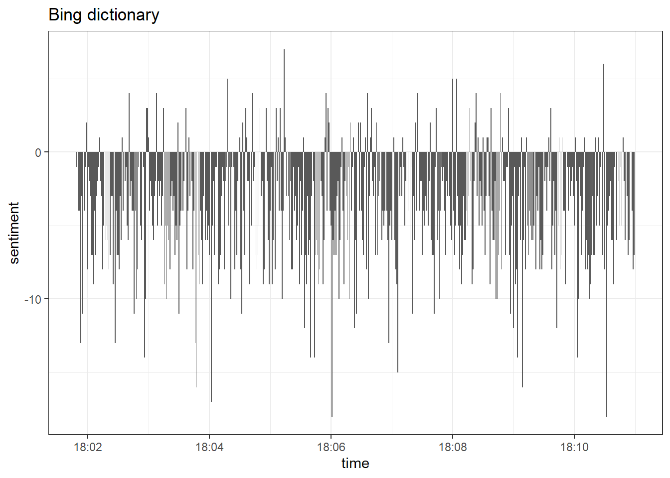

Overall, the tone of tweets is negative. Only a few tweets have a positive valence. Let’s check whether these results are characteristic for the bing dictionary and compare them to another dictionary, namely the afinn dictionary. Let’s load the afinn dictionary next. It’s included in the tidytext package, so you can agree to the licence and load it that way. I have added the afinn dictionary to a .csv to import it more effortlessly, so I’ll use this approach.

afinn <- read.csv("afinn_dictionary.csv")

data_tknzd %>%
  inner_join(afinn) %>%
  group_by(time) %>% 
  summarize(sentiment = sum(value)) %>% 
  ggplot(aes(x = time, y = sentiment)) +
  labs(title = "Afinn dictionary") +
  theme_bw() +
  geom_col(show.legend = FALSE)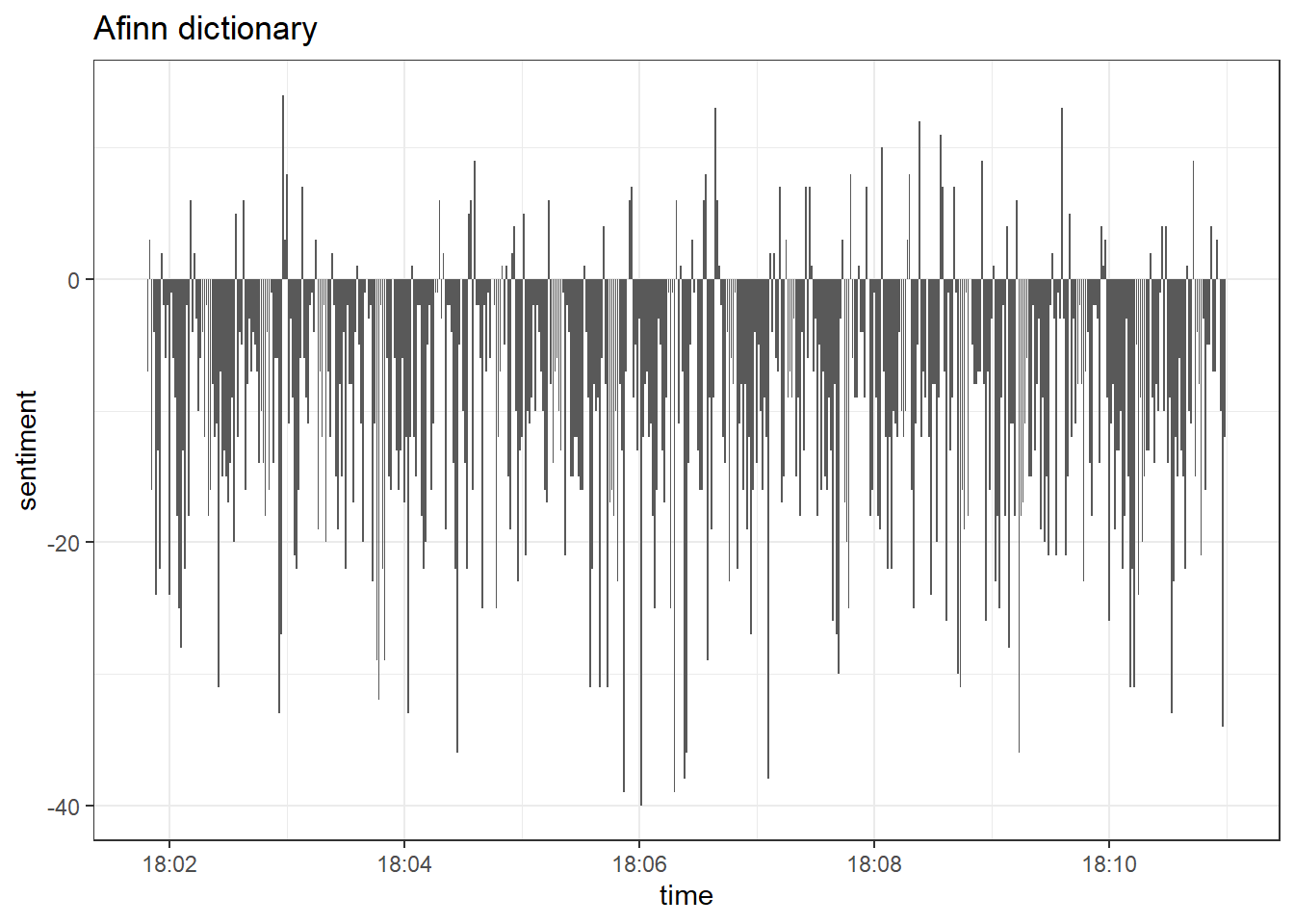

Even though both dictionaries produce similar results, we can see that afinn estimates a greater amount of positive tweets, while the bing dictionary estimates larger blocks of uninterrupted negative sentiment. This behavior of both dictionaries is known, for instance, see this quote:

“Different lexicons for calculating sentiment give results that are different in an absolute sense but have similar relative trajectories . . . The AFINN lexicon gives the largest absolute values, with high positive values. The lexicon from Bing et al. has lower absolute values and seems to label larger blocks of contiguous positive or negative text.” (Silge & Robinson, Link)

Finally, other options include the nrc dictionary that can can estimate 1) negative and positive valence or 2) emotions such anger, sadness, joy, etc. For now, let’s import the valence word lists from nrcand repeat our analysis one last time.

nrc <- read.csv("nrc_dictionary.csv")

nrc <- nrc %>% 
  filter(sentiment == "positive" | sentiment == "negative")

data_tknzd %>%
  inner_join(nrc) %>%
  count(sentiment, time) %>%
  pivot_wider(names_from = sentiment, values_from = n, values_fill = 0) %>%
  mutate(sentiment = positive - negative) %>%
  ggplot(aes(x = time, y = sentiment)) +
  labs(title = "NRC dictionary") +
  theme_bw() +
  geom_col(show.legend = FALSE)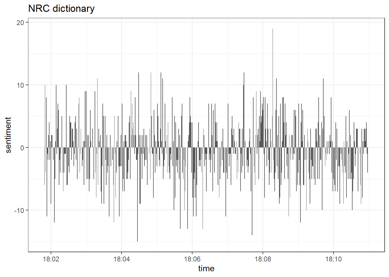

Obviously, the nrc dictionary estimates a much greater amount of positive tweets than bing and afinn. This is why you should handle dictionary-based approaches carefully. As Pipal et al. (2022) put it:

“Many widely used tools for sentiment analysis have been developed by psychologists to measure emotions in free-form writing (such as in product reviews and micro blogs) in the form of pre-defined lexicons (e.g. Tausczik and Pennebaker 2010), yet they are often conveniently used to measure complex latent constructs in highly structured news articles and speeches despite the content-dependent nature of the tools (Puschmann and Powell 2018; Pipal, Schoonvelde, and Schumacher 2022). Different tools embody different methodological assumptions and particular contexts within which they are initially developed from, leading to diverging consequences across different tools.”

To this day, most dictionaries cannot compete with manual annotation. Therefore you should manually validate the estimations before applying sentiment tools to your use case. For a very good comparison between dictionaries and manual annotation, see this article: Link.

Two hands-on learnings: 1) Don’t trust sentiment analyses of pre-designed sentiment reports too much. If you don’t know how these sentiment scores were produced and how reliable those estimations are, you can’t evaluate their quality. 2) My suggestion is that you tailor your own dictionary to your specific use case (e.g., for your company some words might be positive that are negative for other companies) and validate it with manual coding until you are satisfied with its reliability. This is a one-time effort that can really pay-off, especially for smaller businesses.

Practice: Sentiment over time

Alright, we are ready to perform a sentiment analysis for the Kliemann data. Again, we cannot use the tidytext dictionaries because they were developed only for the English language. However, I’ve prepared a German dictionary for you that is based on this article by Christian Rauh. You can find the dictionary as a .csv on Moodle. Use it to analyze the sentiment of the Kliemann data over time. Hint: You will need to follow the sum(value) approach that I used on the afinn dictionary because the dictionary comes with a value column (metric variable) instead of a sentiment column (nominal variable).

Tip for advanced students: One big problem with the above presented dictionary approaches is that they do not take into account sentence structure, but treat each sentence as a bag of words. For those dictionary-approaches, word order does not matter to transport sentiment. If you want to run more complex sentiment analyses in the future, try the vader package. vader is not just dictionary-based, but it is so a so-called “rule-based sentiment analysis tool”. This means that it takes into account sentence structure, e.g., negations. We all agree that “not cute” transports a negative sentiment, but the above presented dictionary approaches treat “not” as a stop word and evaluate “cute” as positive.

8.4.2 Sentiment over time periods

You can define time periods and get the sentiment for each individual time frame. Let’s create three time periods (1 = first 3 min, 2 = 3rd to 6th min, 3 = whole 10 min) and compare the sentiment that both bing and afinn estimate for these three time periods.

Here are the results for bing:

library(lubridate)

data_tknzd %>%
  inner_join(get_sentiments("bing")) %>%
  mutate(period = case_when(
    time <= ymd_hms('2022-02-25 18:03:30') ~ "Period 1",
    time >= ymd_hms('2022-02-25 18:03:31') & 
    time <= ymd_hms('2022-02-25 18:06:30') ~ "Period 2",
    time >= ymd_hms('2022-02-25 18:06:31') & 
    time <= ymd_hms('2022-02-25 18:10:59') ~ "Period 3")) %>% 
  count(period, sentiment)

## # A tibble: 6 × 3
##   period   sentiment     n
##   <chr>    <chr>     <int>
## 1 Period 1 negative    927
## 2 Period 1 positive    513
## 3 Period 2 negative   1697
## 4 Period 2 positive    976
## 5 Period 3 negative   2545
## 6 Period 3 positive   1516

And here are the results for afinn:

library(lubridate)

data_tknzd %>%
  inner_join(afinn) %>%
  mutate(period = case_when(
    time <= ymd_hms('2022-02-25 18:03:30') ~ "Period 1",
    time >= ymd_hms('2022-02-25 18:03:31') & 
    time <= ymd_hms('2022-02-25 18:06:30') ~ "Period 2",
    time >= ymd_hms('2022-02-25 18:06:31') & 
    time <= ymd_hms('2022-02-25 18:10:59') ~ "Period 3")) %>%
  mutate(sentiment = case_when(
    value < 0 ~ "negative",
    value > 0 ~ "positive"
  )) %>%
  count(period, sentiment)

## # A tibble: 6 × 3
##   period   sentiment     n
##   <chr>    <chr>     <int>
## 1 Period 1 negative   1238
## 2 Period 1 positive    743
## 3 Period 2 negative   2182
## 4 Period 2 positive   1301
## 5 Period 3 negative   3301
## 6 Period 3 positive   2033

Practice: Sentiment over time periods

Using the German SentiWS_Rauh dictionary, try to do a similar analysis with the Kliemann data and investigate the sentiment for each individual month starting and ending with the 6th day of this month. Our data from stretches from 6th of May to 3rd of July, so you have to include these three days of July in the June time period.

8.4.3 Sentiment of individual users

Now we can calculate the sentiment for each individual user. Let’s try it.

data_tknzd_bing <- data_tknzd_bing %>%
  count(user, sentiment, time) %>%
  pivot_wider(names_from = sentiment, values_from = n, values_fill = 0) %>% 
  mutate(sentiment = positive - negative)

data_tknzd_bing %>%
  filter(user == "common_sense54" | user == "EdCutter1" | user == "BaloIreen" | user == "LateNighter5")

## # A tibble: 63 × 5
##    user      time                negative positive sentiment
##    <chr>     <dttm>                 <int>    <int>     <int>
##  1 BaloIreen 2022-02-25 18:02:33        1        2         1
##  2 BaloIreen 2022-02-25 18:02:51        1        2         1
##  3 BaloIreen 2022-02-25 18:02:59        1        2         1
##  4 BaloIreen 2022-02-25 18:03:07        1        2         1
##  5 BaloIreen 2022-02-25 18:03:21        1        2         1
##  6 BaloIreen 2022-02-25 18:03:34        1        2         1
##  7 BaloIreen 2022-02-25 18:03:44        1        2         1
##  8 BaloIreen 2022-02-25 18:09:01        1        2         1
##  9 BaloIreen 2022-02-25 18:09:28        1        2         1
## 10 BaloIreen 2022-02-25 18:06:08        0        1         1
## # … with 53 more rows

…and turn it into a visualization of our most active users over time:

data_tknzd_bing %>% 
  group_by(user, time) %>%
  filter(user == "common_sense54" | user == "EdCutter1" | user == "BaloIreen" | user == "LateNighter5") %>%
  ggplot(aes(x = time, y = sentiment, fill = user)) +
  geom_col(show.legend = FALSE) +
  labs(title = "Bing: The sentiment of the most active users") +
  theme_bw() +
  facet_wrap(~user)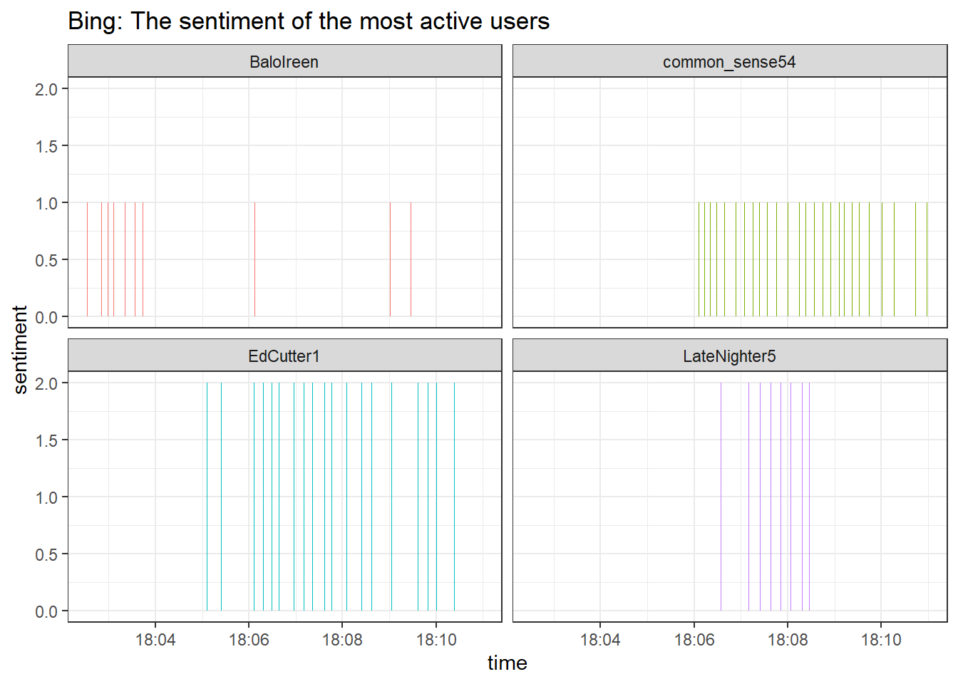

According to the bing dictionary the sentiment of our most active twitter users was positive and stayed positive over the 10-minute time frame that we are currently looking at. Positive sentiment while talking about the outbreak of war? Those are odd results. Maybe the positive sentiment is characteristic of more active users?

data_tknzd %>%
  inner_join(get_sentiments("bing")) %>%
  count(sentiment, time) %>%
  pivot_wider(names_from = sentiment, values_from = n, values_fill = 0) %>% 
  mutate(sentiment = positive - negative) %>%
  ggplot(aes(x = time, y = sentiment)) +
  labs(title = "Bing dictionary") +
  theme_bw() +
  geom_col(show.legend = FALSE)

Overall, the tone of tweets is negative, which implies that the most active users are characterized by a more positive sentiment. That’s an interesting result and might be an indicator that very active accounts are trying to push the public opinion in some specific direction. We could run more in-depth analyses of more users and longer time-periods to prove that, but for now we want to focus on alternative dictionaries.

Knowing this, let’s check how similar the results are for our most active users.

data_tknzd %>% 
  inner_join(afinn) %>%
  group_by(user, time) %>%
  summarize(sentiment = sum(value)) %>%
  filter(user == "common_sense54" | user == "EdCutter1" | user == "BaloIreen" | user == "LateNighter5") %>%
  ggplot(aes(x = time, y = sentiment, fill = user)) +
  geom_col(show.legend = FALSE) +
  labs(title = "Afinn: The sentiment of the most active users") +
  theme_bw() +
  facet_wrap(~user)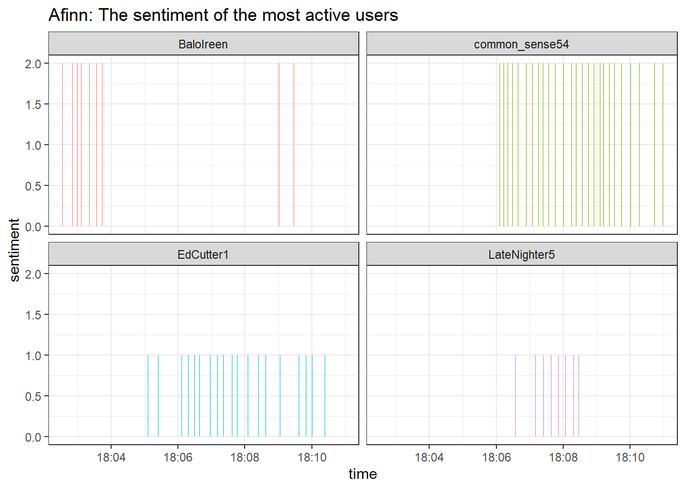

That looks good, both bing and afinn come to similar conclusions, i.e., the most active users publish tweets with a positive sentiment. The dictionary approaches that treat sentiment as the sum of the individual negativity/emotion ratings of words are consistent with each other.

8.5 Take-Aways

• Text normalization: You can perform the entire preprocessing of your documents using the tidy text approach (tokenization, stop words, removal, etc.).
• Word freqencies & Log Odds: The tidy text approach can also be used to calculate word frequencies and log odds to identify the most common word per author, etc.
• Topic modeling: Topic models are mixed-membership models, i.e., they assume that every text contains a mix of different topics. The best known topic modeling algorithm is LDA.
• K: Number of topics to be estimated.
• Word-topic matrix: Aids in the creation of topic-specific word lists.
• Document-topic matrix: Aids in the creation of document-specific topic lists.

8.6 Additional tutorials

You still have questions? The following tutorials, books, & papers may help you:

• Video Introduction to Topic Modeling by C. Bail
• Blog about Topic Modeling by C. Bail
• Blog about Interpreting Topic Models (STM + tidytext style) by J. Silge
• Text as Data by V. Hase, Tutorial 13
• Text Mining in R. A Tidy Approach by Silge & Robinson (2017)
• Video Introduction to Evaluating Topic Models (in Python!)

---

4. To disable this feature, use the to_lower = FALSE option.↩︎