Solutions

This is where you’ll find solutions for all of the tutorials.

Solutions for Exercise 1

Task 1

Below you will see multiple choice questions. Please try to identify the correct answers. 1, 2, 3 and 4 correct answers are possible for each question.

1. What panels are part of RStudio?

Solution:

• source (x)
• console (x)
• packages, files & plots (x)

2. How do you activate R packages after you have installed them?

Solution:

• library() (x)

3. How do you create a vector in R with elements 1, 2, 3?

Solution:

• c(1,2,3) (x)

4. Imagine you have a vector called ‘vector’ with 10 numeric elements. How do you retrieve the 8th element?

Solution:

• vector[8] (x)

5. Imagine you have a vector called ‘hair’ with 5 elements: brown, black, red, blond, other. How do you retrieve the color ‘blond’?

Solution:

• hair[4] (x)

Task 2

Create a numeric vector with 8 values and assign the name age to the vector. First, display all elements of the vector. Then print only the 5th element. After that, display all elements except the 5th. Finally, display the elements at the positions 6 to 8.

Solution:

age <- c(65,52,73,71,80,62,68,87)
age

## [1] 65 52 73 71 80 62 68 87

age[5]

## [1] 80

age[-5]

## [1] 65 52 73 71 62 68 87

age[6:8]

## [1] 62 68 87

Task 3

Create a non-numeric, i.e. character, vector with 4 elements and assign the name eye_color to the vector. First, print all elements of this vector to the console. Then have only the value in the 2nd element displayed, then all values except the 2nd element. At the end, display the elements at the positions 2 to 4.

Solution:

eye_color <- c("blue", "green", "brown", "other")
eye_color

## [1] "blue"  "green" "brown" "other"

eye_color[2]

## [1] "green"

eye_color[-2]

## [1] "blue"  "brown" "other"

eye_color[2:4]

## [1] "green" "brown" "other"

Task 4

Get the “data_tutorial2.csv” from Moodle ( 02. November material folder ) and put it into the folder that you want to use as working directory.

Set your working directory and load the data into R by saving it into a source object called data. Note: This time, it’s a csv that is actually separated by commas, not by semicolons.

Solution:

setwd("C:/Users/LaraK/Documents/IPR/")
data <- read.csv("data_tutorial2.csv", header = TRUE)

Task 5

Now, print only the age column to the console. Use the $ operator first. Then try to achieve the same result using the subsetting operators, i.e. [].

Solution:

data$age # first version

##  [1] 20 25 29 22 25 26 26 27  8 26 27 26 25 27 29 26 21 23 24 26

data[,2] # second version

##  [1] 20 25 29 22 25 26 26 27  8 26 27 26 25 27 29 26 21 23 24 26

Task 6

Print only the first 6 age numbers to the console. Use the $ operator first. Then try to achieve the same result using the subsetting operators, i.e. [].

Solution:

data$age[1:6] # first version

## [1] 20 25 29 22 25 26

data[1:6,2] # second version

## [1] 20 25 29 22 25 26

Solutions for Exercise 2

Task 1

Below you will see multiple choice questions. Please try to identify the correct answers. 1, 2, 3 and 4 correct answers are possible for each question.

1. What are the main characteristics of tidy data?

Solution:

• Every observation is a row. (x)

2. What are dplyr functions?

Solution:

• mutate() (x)

3. How can you sort the eye_color of Star Wars characters from Z to A?

Solution:

• starwars_data %>% arrange(desc(eye_color)) (x)
• starwars_data %>% select(eye_color) %>% arrange(desc(eye_color))

4. Imagine you want to recode the height of the these characters. You want to have three categories from small and medium to tall. What is a valid approach?

Solution:

• starwars_data %>% mutate(height = case_when(height<=150~"small",height<=190~"medium",height>190~"tall"))

5. Imagine you want to provide a systematic overview over all hair colors and what species wear these hair colors frequently (not accounting for the skewed sampling of species)? What is a valid approach?

Solution:

• starwars_data %>% group_by(hair_color, species) %>% summarize(count = n()) %>% arrange(hair_color)

Task 2

Now it’s you turn. Load the starwars data like this:

library(dplyr)              # to activate the dplyr package
starwars_data <- starwars   # to assign the pre-installed starwars data set (dplyr) into a source object in our environment

How many humans are contained in the starwars data overall? (Hint: use summarize(count = n()) or count())?

Solution:

You can use summarize(count = n()):

starwars_data %>%
  filter(species == "Human") %>% 
  summarize(count = n())

## # A tibble: 1 × 1
##   count
##   <int>
## 1    35

Alternatively, you can use the count() function:

starwars_data %>%
  filter(species == "Human") %>% 
  count(species)

## # A tibble: 1 × 2
##   species     n
##   <chr>   <int>
## 1 Human      35

Task 3

How many humans are contained in starwars by gender?

Solution:

You can use summarize(count = n()):

starwars_data %>%
  filter(species == "Human") %>% 
  group_by(species, gender) %>% 
  summarize(count = n())

## # A tibble: 2 × 3
## # Groups:   species [1]
##   species gender    count
##   <chr>   <chr>     <int>
## 1 Human   feminine      9
## 2 Human   masculine    26

Alternatively, you can use the count() function:

starwars_data %>%
  filter(species == "Human") %>% 
  count(species, gender)

## # A tibble: 2 × 3
##   species gender        n
##   <chr>   <chr>     <int>
## 1 Human   feminine      9
## 2 Human   masculine    26

Task 4

What is the most common eye_color among Star Wars characters? (Hint: use arrange())__

Solution:

starwars_data %>%
  group_by(eye_color) %>% 
  summarize(count = n()) %>%
  arrange(desc(count))

## # A tibble: 15 × 2
##    eye_color     count
##    <chr>         <int>
##  1 brown            21
##  2 blue             19
##  3 yellow           11
##  4 black            10
##  5 orange            8
##  6 red               5
##  7 hazel             3
##  8 unknown           3
##  9 blue-gray         1
## 10 dark              1
## 11 gold              1
## 12 green, yellow     1
## 13 pink              1
## 14 red, blue         1
## 15 white             1

Task 5

What is the average mass of Star Wars characters that are not human and have yellow eyes? (Hint: remove all NAs)__

Solution:

starwars_data %>%
  filter(species != "Human" & eye_color=="yellow") %>%
  summarize(mean_mass = mean(mass, na.rm=TRUE))

## # A tibble: 1 × 1
##   mean_mass
##       <dbl>
## 1      74.1

Task 6

Compare the mean, median, and standard deviation of mass for all humans and droids. (Hint: remove all NAs)__

Solution:

starwars_data %>%
  filter(species=="Human" | species=="Droid") %>%
  group_by(species) %>%                                
  summarize(M = mean(mass, na.rm = TRUE),
            Med = median(mass, na.rm = TRUE),
            SD = sd(mass, na.rm = TRUE)
            )

## # A tibble: 2 × 4
##   species     M   Med    SD
##   <chr>   <dbl> <dbl> <dbl>
## 1 Droid    69.8  53.5  51.0
## 2 Human    82.8  79    19.4

Task 7

Create a new variable in which you store the mass in gram. Add it to the data frame.

Solution:

starwars_data <- starwars_data %>%
  mutate(gr_mass = mass*1000)

starwars_data %>% 
  select(name, species, mass, gr_mass)

## # A tibble: 87 × 4
##    name               species  mass gr_mass
##    <chr>              <chr>   <dbl>   <dbl>
##  1 Luke Skywalker     Human      77   77000
##  2 C-3PO              Droid      75   75000
##  3 R2-D2              Droid      32   32000
##  4 Darth Vader        Human     136  136000
##  5 Leia Organa        Human      49   49000
##  6 Owen Lars          Human     120  120000
##  7 Beru Whitesun lars Human      75   75000
##  8 R5-D4              Droid      32   32000
##  9 Biggs Darklighter  Human      84   84000
## 10 Obi-Wan Kenobi     Human      77   77000
## # … with 77 more rows

Solutions for Exercise 3

Task 1

Try to reproduce this plot with dplyr and ggplot2. (Hint: You can hide the legend by adding theme(legend.position = "none") to your plot.)

Solution:

data %>% 
  mutate(sex = case_when(
    sex == 0 ~ "Female",
    sex == 1 ~ "Male")) %>%
  mutate(Party = case_when(
    partyid == 1 ~ "Democrat",
    partyid == 2 ~ "Independent",
    partyid == 3 ~ "Republican")) %>%
  ggplot(aes(x=Party,y=negemot, fill=Party)) +
  stat_summary(geom = "bar", fun = "mean") +
  theme_bw() +
  theme(legend.position = "none") +
  labs(title = "Climate change attitudes of U.S. partisans by gender",
       y = "Negative emotions about climate change") +
  facet_wrap(~sex, nrow=2)

Task 2

Now, try to reproduce this graph. (Hint: You will need to recode the ideology variable in a way that higher values represent stronger attitudes, independent of partisanship.)

Solution:

data <- data %>% 
  mutate(ideology_ext = case_when(
    ideology == 1 ~ 4,
    ideology == 2 ~ 3,
    ideology == 3 ~ 2,
    ideology == 4 ~ 1,
    ideology == 5 ~ 2,
    ideology == 6 ~ 3,
    ideology == 7 ~ 4)) %>%
  mutate(sex = case_when(
    sex == 0 ~ "Female",
    sex == 1 ~ "Male")) %>%
  mutate(Party = case_when(
    partyid == 1 ~ "Democrat",
    partyid == 2 ~ "Independent",
    partyid == 3 ~ "Republican"))

data %>% 
  ggplot(aes(x=Party,y=ideology_ext, fill=Party)) +
  geom_boxplot() +
  theme_bw() +
  theme(legend.position = "none") +
  labs(title = "Ideological extremity of U.S. partisans by gender",
       y = "Ideological extremity") +
  facet_wrap(~sex)

Task 3

Can you make a chart that breaks down the relationship between age, negative emotions about climate change, and ideological extremity for the different sexes AND parties?

Solution 1:

data %>%
  ggplot(aes(x=age,y=negemot, size=ideology_ext, color = Party)) +
  geom_point() +
  scale_size(range = c(0.3, 3), name = "Ideological extremity") +  # You can't guess the exact value that I've used here. Just use whatever looks good for you and comes close to the solution.
  theme_bw() +
  labs(title = "Relationship between age, climate change attitudes, \n and ideological extremity",
       x = "Age", y = "Negative emotions about climate change") +
  facet_wrap(~sex, nrow=2)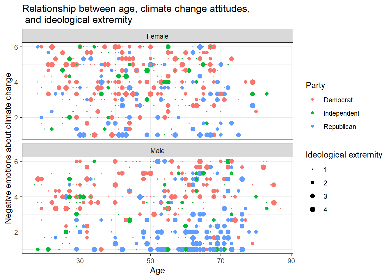

Solution 2:

Alternatively, you might enjoy this look that you can create with facet_grid():

data %>% 
  ggplot(aes(x=age,y=negemot, size=ideology_ext, color = Party)) +
  geom_point() +
  scale_size(range = c(0.3, 3), name = "Ideological extremity") +
  theme_bw() +
  labs(title = "Relationship between age, climate change attitudes, and ideological extremity",
       x = "Age", y = "Negative emotions about climate change") +
  facet_grid(vars(sex), vars(Party))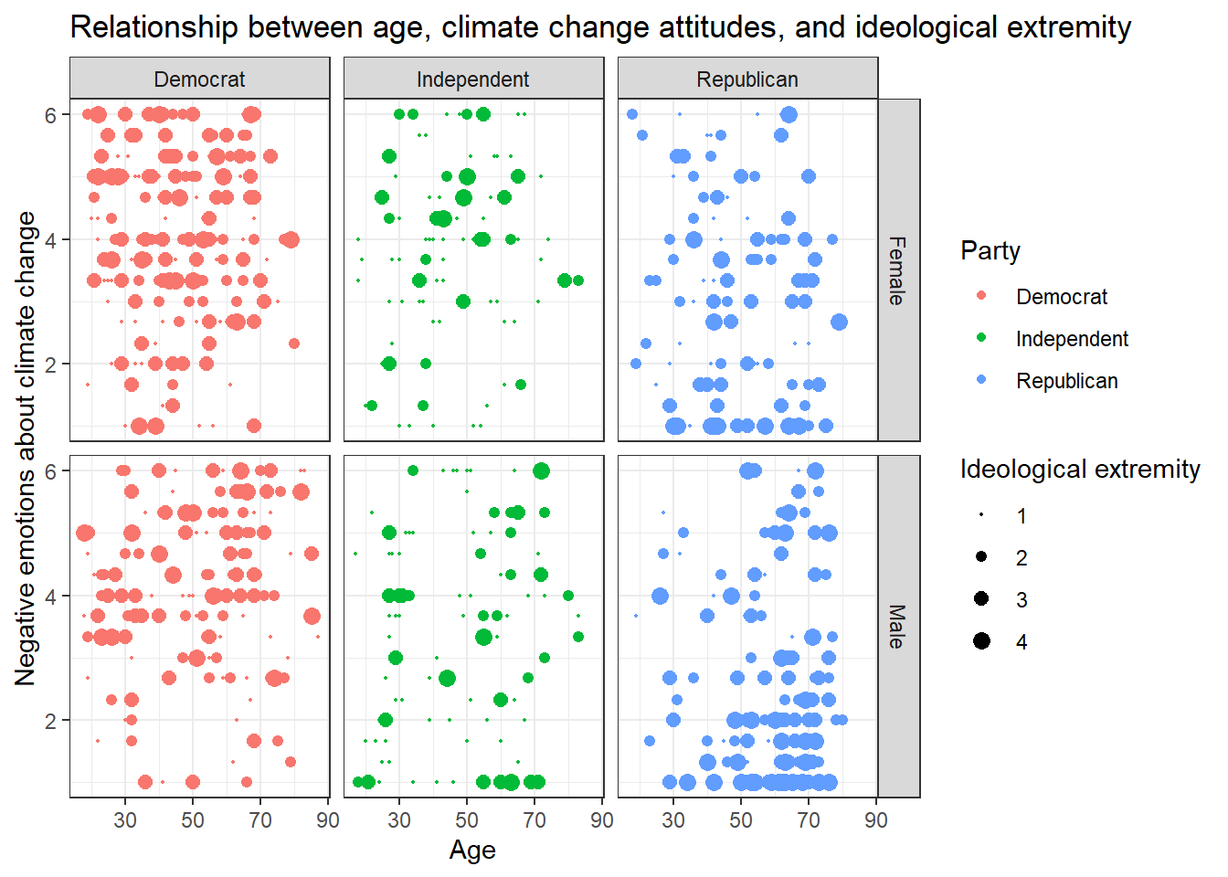

Solution 3:

Or even this look, also done with facet_grid():

data %>% 
  ggplot(aes(x=age,y=negemot, size=ideology_ext, color = Party)) +
  geom_point() +
  scale_size(range = c(0.3, 3), name = "Ideological extremity") +
  theme_bw() +
  labs(title = "Relationship between age, climate change attitudes, and ideological extremity",
       x = "Age", y = "Negative emotions about climate change") +
  facet_grid(~sex + Party)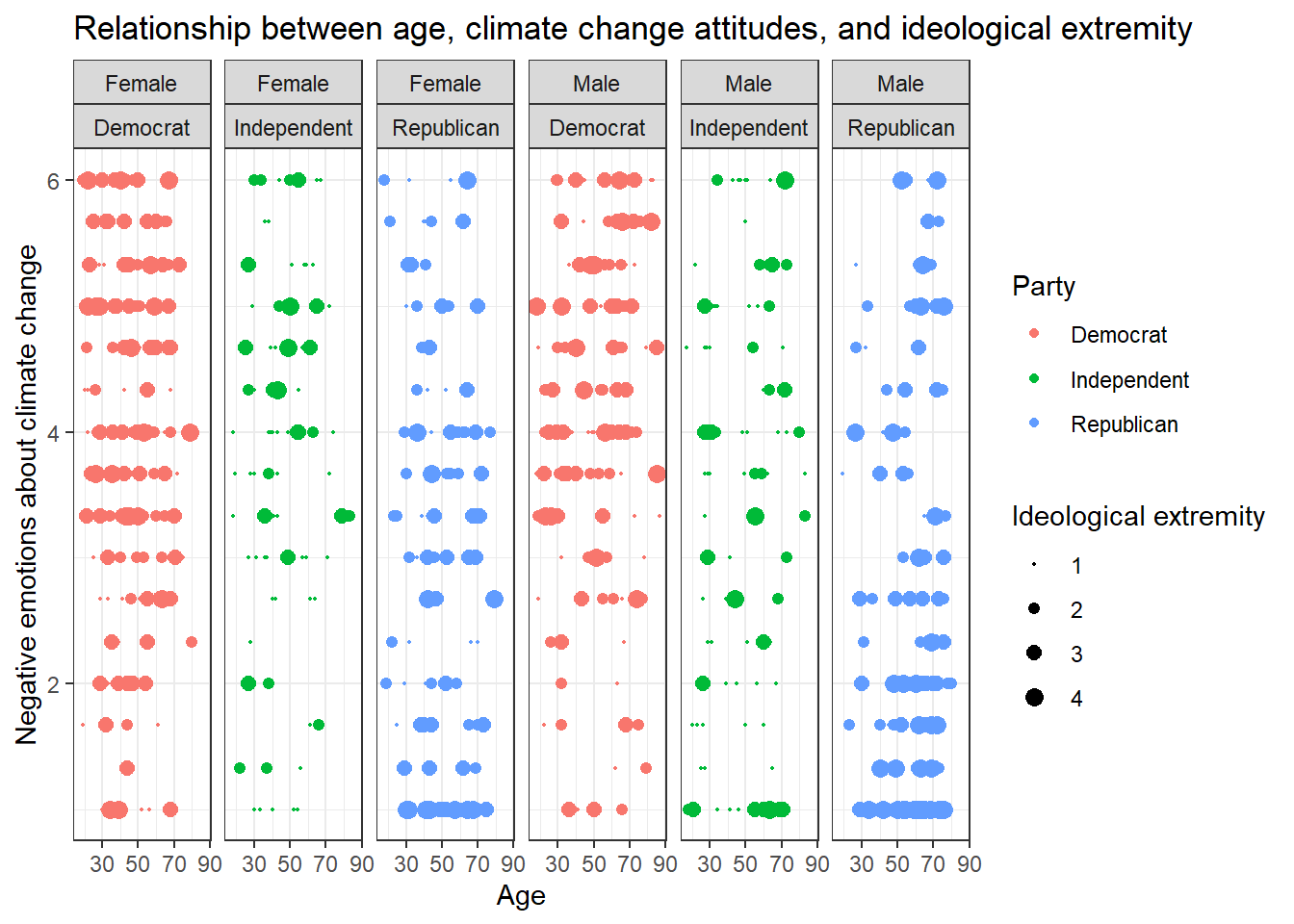

Solutions for Exercise 4

This exercise was created because some students asked to get some more practice. You don’t have to work through it, but it can certainly help you with the graded assignment. In this exercise, we will work with the mtcars data that comes pre-installed with dplyr.

library(tidyverse)

data <- mtcars

# To make the data somewhat more interesting, let's set a few values to missing values:
data$wt <- na_if(data$wt, 4.070)
data$mpg <- na_if(data$mpg, 22.8)

Task 1

Check the data set for missing values (NAs) and delete all observations that have missing values.

Solution:

You can solve this by excluding NAs in every single column:

data <- data %>%
  # we'll now only keep observations that are NOT NAs in the following variables (remember that & = AND):
  filter(!is.na(mpg) & !is.na(cyl) & !is.na(disp) & !is.na(hp) & !is.na(drat) & !is.na(wt) & !is.na(qsec)
         & !is.na(vs) & !is.na(am) & !is.na(gear) & !is.na(carb))

Alternatively, excluding NAs from the entire data set works, too, but you have not learned the na_omit()function in the tutorials:

data <- data %>%
  na.omit()

Task 2

Let’s transform the weight wt of the cars. Currently, it’s given as Weight in 1000 lbs. I guess you are not used to lbs, so try to mutate wt to represent Weight in 1000 kg. 1000 lbs = 453.59 kg, so we will need to divide by 2.20.

Similarly, I think that you are not very familiar with the unit Miles per gallon of the mpg variable. Let’s transform it into Kilometer per liter. 1 m/g = 0.425144 km/l, so again divide by 2.20.

Solution:

data <- data %>%
  mutate(wt = wt/2.20)

data <- data %>%
  mutate(mpg = mpg/2.20)

Task 3

Now we want to group the weight of the cars in three categories: light, medium, heavy. But how to define light, medium, and heavy cars, i.e., at what kg should you put the threshold? A reasonable approach is to use quantiles (see Tutorial: summarize() [+ group_by()]). Quantiles divide data. For example, the 75% quantile states that exactly 75% of the data values are equal or below the quantile value. The rest of the values are equal or above it.

Use the lower quantile (0.25) and the upper quantile (0.75) to estimate two values that divide the weight of the cars in three groups. What are these values?

Solution:

data %>% 
  summarize(UQ_wt= quantile(wt, 0.75),
            LQ_wt= quantile(wt, 0.25))

##      UQ_wt    LQ_wt
## 1 1.622727 1.190909

75% of all cars weigh 1.622727* 1000kg or less and 25% of all cars weigh 1.190909* 1000kg or less.

Task 4

Use the values from Task 3 to create a new variable wt_cat that divides the cars in three groups: light, medium, and heavy cars.

Solution:

data <- data %>% 
  mutate(wt_cat = case_when(
    wt <= 1.190909 ~ "light car",
    wt < 1.622727 ~ "medium car",
    wt >= 1.622727 ~ "heavy car"))

Task 5

How many light, medium, and heavy cars are part of the data?

Solution:

You can solve this with the summarize(count = n() function:

data %>% 
  group_by(wt_cat) %>% 
  summarize(count = n())

## # A tibble: 3 × 2
##   wt_cat     count
##   <chr>      <int>
## 1 heavy car      9
## 2 light car      7
## 3 medium car    13

9 heavy cars, 13 medium cars, and 7 light cars.

Alternatively, you can also use the count() function:

data %>% 
  count(wt_cat)

##       wt_cat  n
## 1  heavy car  9
## 2  light car  7
## 3 medium car 13

Task 6

Now sort this count of the car weight classes from highest to lowest.

Solution:

data %>% 
  group_by(wt_cat) %>% 
  summarize(count = n()) %>% 
  arrange(desc(count))

## # A tibble: 3 × 2
##   wt_cat     count
##   <chr>      <int>
## 1 medium car    13
## 2 heavy car      9
## 3 light car      7

Task 7

Make a scatter plot to indicate how many km per liter (mpg) a car can drive depending on its weight (wt). Facet the plot by weight class (wt_cat). Try to hide the plot legend (you have learned that in another exercise).

data %>% 
  mutate(wt_cat = factor(wt_cat, levels = c("light car", "medium car", "heavy car"))) %>% 
  ggplot(aes(x=wt, y=mpg, color=wt_cat)) +
  geom_point() +
  theme_bw() +
  scale_color_manual(values = c("#7b3294", "#84798a", "#008837")) +  # optional command, choose your own beautiful colors for the graph
  theme(legend.position = "none") +
  labs(title = "Relationship between car weight and achieved kilometers per liter", x="Weight in 1000kg", y="km/l") +
  facet_wrap(~wt_cat)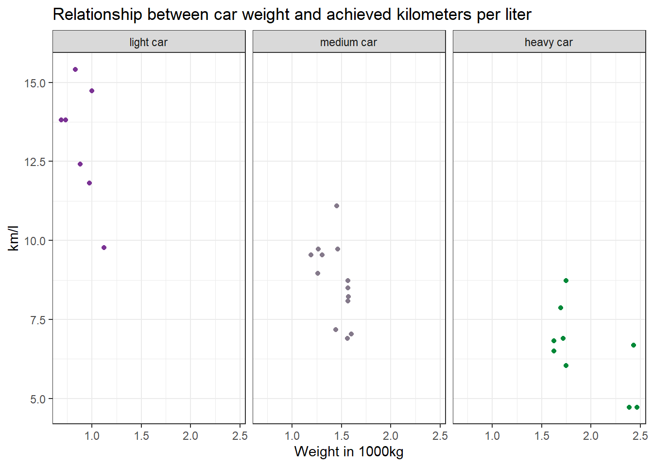

Task 8

Recreate the diagram from Task 7, but exclude all cars that weigh between 1.4613636 and 1.5636364 *1000kg from it.

Solution:

data %>%
  filter(wt < 1.4613636 | wt > 1.5636364) %>% 
  mutate(wt_cat = factor(wt_cat, levels = c("light car", "medium car", "heavy car"))) %>% 
  ggplot(aes(x=wt, y=mpg, color=wt_cat)) +
  geom_point() +
  theme_bw() +
  scale_color_manual(values = c("#7b3294", "#84798a", "#008837")) + # optional command, choose your own beautiful colors for the graph
  theme(legend.position = "none") +
  labs(title = "Relationship between car weight and achieved kilometers per liter", x="Weight in 1000kg", y="km/l") +
  facet_wrap(~wt_cat)

Why would we use data %>% filter(wt < 1.4613636 | wt > 1.5636364) instead of data %>% filter(wt > 1.4613636 | wt < 1.5636364)?

Let’s look at the resulting data sets when you apply those filters to compare them:

data %>%
  select(wt) %>% 
  filter(wt < 1.4613636 | wt > 1.5636364)

##                            wt
## Mazda RX4           1.1909091
## Mazda RX4 Wag       1.3068182
## Valiant             1.5727273
## Duster 360          1.6227273
## Merc 240D           1.4500000
## Merc 450SL          1.6954545
## Merc 450SLC         1.7181818
## Cadillac Fleetwood  2.3863636
## Lincoln Continental 2.4654545
## Chrysler Imperial   2.4295455
## Fiat 128            1.0000000
## Honda Civic         0.7340909
## Toyota Corolla      0.8340909
## Toyota Corona       1.1204545
## Dodge Challenger    1.6000000
## Camaro Z28          1.7454545
## Pontiac Firebird    1.7477273
## Fiat X1-9           0.8795455
## Porsche 914-2       0.9727273
## Lotus Europa        0.6877273
## Ford Pantera L      1.4409091
## Ferrari Dino        1.2590909
## Maserati Bora       1.6227273
## Volvo 142E          1.2636364

The resulting table does not include any cars that weigh between 1.4613636 and 1.5636364. But if you use data %>% filter(wt > 1.4613636 | wt < 1.5636364)…

data %>%
  select(wt) %>% 
  filter(wt > 1.4613636 | wt < 1.5636364)

##                            wt
## Mazda RX4           1.1909091
## Mazda RX4 Wag       1.3068182
## Hornet 4 Drive      1.4613636
## Hornet Sportabout   1.5636364
## Valiant             1.5727273
## Duster 360          1.6227273
## Merc 240D           1.4500000
## Merc 280            1.5636364
## Merc 280C           1.5636364
## Merc 450SL          1.6954545
## Merc 450SLC         1.7181818
## Cadillac Fleetwood  2.3863636
## Lincoln Continental 2.4654545
## Chrysler Imperial   2.4295455
## Fiat 128            1.0000000
## Honda Civic         0.7340909
## Toyota Corolla      0.8340909
## Toyota Corona       1.1204545
## Dodge Challenger    1.6000000
## AMC Javelin         1.5613636
## Camaro Z28          1.7454545
## Pontiac Firebird    1.7477273
## Fiat X1-9           0.8795455
## Porsche 914-2       0.9727273
## Lotus Europa        0.6877273
## Ford Pantera L      1.4409091
## Ferrari Dino        1.2590909
## Maserati Bora       1.6227273
## Volvo 142E          1.2636364

… cars that weigh between 1.4613636 and 1.5636364 are still included!

But why? The filter()function always keeps cases based on the criteria that you provide.

In plain English, my solution code says the following: Take my dataset “data” and keep only those cases where the weight variable wt is less than 1.4613636 OR larger than 1.5636364. Put differently, the solution code says: Delete all cases that are greater than 1.4613636 but are also less than 1.5636364.

The wrong code, on the other hand, says: Take my dataset “data” and keep only those cases where the weight variable wt is greater than 1.4613636 OR smaller than 1.5636364. This is ALL the data because all your cases will be greater than 1.4613636 OR smaller than 1.5636364. You are not excluding any cars.

Solutions for Exercise 5

First, load the library stringr (or the entire tidyverse).

library(tidyverse)

We will work on real data in this exercise. But before that, we will test our regex on a simple “test” vector that contains hyperlinks of media outlets and webpages. So run this code and create a vector called “seitenURL” in your environment:

seitenURL <- c("https://www.bild.de", "https://www.kicker.at/sport", "http://www.mycoffee.net/fresh", "http://www1.neuegedanken.blog", "https://home.1und1.info/magazine/unterhaltung", "https://de.sputniknews.com/technik", "https://rp-online.de/nrw/staedte/geldern", "https://www.bzbasel.ch/limmattal/region-limmattal", "http://sportdeutschland.tv/wm-maenner-2019")

Task 1

Let’s get rid of the first part of the URL strings in our “seitenURL” vector, i.e., everything that comes before the name of the outlet (You will need to work with str_replace). Usually, this is some kind of version of “https://www.” or “http://www.” Try to make your pattern as versatile as possible! In a big data set, there will always be exceptions to the rule (e.g., “http://sportdeutschland.tv”), so try to match regex–i.e., types of characters instead of real characters–as often as you can!

seitenURL <-str_replace(seitenURL, "^(http)(s?)[:punct:]{3}(www[:punct:]|www1[:punct:]|w?)", "")
# this matches all strings that start with http: '^(http)'
# this matches all strings that are either http or https: (s?) -> because '?' means "zero or more"
# followed by exactly one dot and two forwardslashes: '[:punct:]{3}'
# followed by either a www.: '(www[:punct:]'
# or followed by a www1.: '|www1[:punct:])'
# or not followed by any kind of www (this is necessary for the rp-online-URL): 'w?'
# and replaces the match with nothing, i.e., an empty string: ', ""'

Task 2

Using the seitenURL vector, try to get rid of the characters that follow the media outlet (e.g., “.de” or “.com”).

seitenURL <- str_replace(seitenURL, "[:punct:]{1}(com|de|blog|net|tv|at|ch|info).*", "")
# this matches all strings that have exactly one dot: "[:punct:]{1}"
# this matches either com, de, blog and many more: "(com|de|blog|net|tv|at|ch)"
# this matches any character zero or multiple times: ".*"

Task 3

Now download our newest data set on Moodle and load it into R as an object called “data”. It is a very reduced version of the original data set that I’ve worked with for a project. The data set investigates what kind of outlets and webpages are most often shared and engaged with on Twitter and Facebook. We have tracked every webpage, from big players like BILD to small, private blogs. However, this is a reduced version of my raw data. The outlets are still hidden in the URLs, so we need to extract them first using the regex patterns that you’ve just created.

Use this command and adapt it with your patterns (it uses str_replace in combination with mutate):

data2 <- data %>%
  mutate(seitenURL = str_replace_all(seitenURL, "^(http)(s?)[:punct:]{3}(www[:punct:]|www1[:punct:]|w?)", "")) %>%
  mutate(seitenURL = str_replace_all(seitenURL, "[:punct:]{1}(com|de|blog|net|tv|at|ch|info).*", ""))

Task 4

The data set provides two additional, highly informative columns: “SeitenAnzahlTwitter” and “SeitenAnzahlFacebook”. These columns show the number of reactions (shares, likes, comments) for each URL. Having extracted the media outlets, let us examine which media outlet got the most engagement on Twitter and Facebook from all their URLs. Utilize your dplyr abilities to create an R object named “overview” that stores the summary statistic (remember group_by and summarize!) of the engagement on Twitter and Facebook per media outlet.

Next, arrange your “overview” data to reveal which media outlet creates the most engagement on Twitter. Do the same for Facebook.

overview <- data2 %>%
  group_by(seitenURL) %>%
  summarize(twitter = sum(seitenAnzahlTwitter),
            facebook = sum(seitenAnzahlFacebook))

overview %>%
  arrange(desc(twitter))

overview %>%
  arrange(desc(facebook))

Solutions for Exercise 6

Task 1: Tokenization

Load the Kliemann data into RStudio. Use the tutorial code and to set the encoding and to convert the date column to a standardized date format. After loading the Kliemann data keep only the time, user, and full_text column.

Next, try to tokenize the data.

Solution:

# First: Load and shorten data
data <- read.csv("Kliemann-full-tweets.csv", encoding = "UTF-8")
data_short <- data %>% 
  select(time, user, full_text)

library(lubridate)

data_short <- data_short %>% 
  mutate(time = lubridate::ymd_hms(time)) %>%
  tibble()

# Second: Tokenize
remove_reg <- "&amp;|&lt;|&gt;"

data_tknzd <- data_short %>%
  mutate(tweet = row_number()) %>%
  filter(!str_detect(full_text, "^RT")) %>%
  mutate(text = str_remove_all(full_text, remove_reg)) %>%
  unnest_tokens(word, full_text, token = "tweets") %>%
  filter(!str_detect(word, "^[:digit:]+$")) %>%
  filter(!str_detect(word, "^http")) %>%
  filter(!str_detect(word, "^(\\+)+$")) %>%
  filter(!str_detect(word, "^(\\+)+(.)+$")) %>%
  filter(!str_detect(word, "^(\\-)+$")) %>%
  filter(!str_detect(word, "^(\\-)+(.)+$")) %>%
  filter(!str_detect(word, "^(.)+(\\+)+$"))

Task 2: Stop word removal

Now it’s your turn. The Kliemann data is in German, so you can’t use the tidytext stop word list, which is meant for English text only. So install and load the ‘stopwords’ package that allows you to create a dataframe that contains German stop words by using this command: stop_word_german <- data.frame(word = stopwords::stopwords("de"), stringsAsFactors = FALSE). Create your German stop word list and use it to remove stop words from your tokens.

Solution:

# First: install and load the stopwords package
if(!require(stopwords)) {
  install.packages("stopwords"); 
  require(stopwords)
} #load / install+load stopwords

# Second: create a stop word list
stop_word_german <- data.frame(word = stopwords::stopwords("de"), stringsAsFactors = FALSE)

# Third: remove German stop words from tokens
data_tknzd <- data_tknzd %>% 
  filter(!word %in% stop_word_german$word)

Optional solution:

If you want to add additional stop words to your stop word list, you can use this solution instead. I would recommend using it, because German stop word lists are often not as advanced as English stop word lists. In addition, they need to be tailored for specific text types, such as colloquial German:

# First: install and load the stopwords package
if(!require(stopwords)) {
  install.packages("stopwords"); 
  require(stopwords)
} #load / install+load stopwords

# Second: create a stop word list
stop_word_german <- data.frame(word = stopwords::stopwords("de"), stringsAsFactors = FALSE)

# Optional: Here you can insert your own stop words, if the German list seems too short for you (231 words against 1149 in English)
stop_word_german <- stop_word_german %>%
  add_row(word = "beim") %>% 
  add_row(word = "and") %>%
  add_row(word = "mehr") %>%
  add_row(word = "ganz") %>%
  add_row(word = "fast") %>%
  add_row(word = "klar") %>%
  add_row(word = "mal") %>%
  add_row(word = "dat") %>%
  add_row(word = "biste") %>%
  add_row(word = "schon") %>%
  add_row(word = "gell")  %>%
  add_row(word = "dass") %>%
  add_row(word = "seit") %>%
  add_row(word = "ja") %>%
  add_row(word = "wohl") %>%
  add_row(word = "gar") %>%
  add_row(word = "ne") %>%
  add_row(word = "sone") %>%
  add_row(word = "dar") %>%
  add_row(word = "ahja") %>%
  add_row(word = "eher") %>%
  add_row(word = "naja") %>%
  add_row(word = "yes") %>%
  add_row(word = "pls") %>%
  add_row(word = "halt") %>%
  add_row(word = "hast") %>%
  add_row(word = "hat") %>%
  add_row(word = "wurde") %>%
  add_row(word = "wurden") %>%
  add_row(word = "wurdest") %>%
  add_row(word = "war") %>%
  add_row(word = "warst") %>%
  add_row(word = "gib") %>%
  add_row(word = "gibst") %>%
  add_row(word = "gibt") %>%
  add_row(word = "entweder") %>%
  add_row(word = "beinahe") %>%
  add_row(word = "ganz") %>%
  add_row(word = "ganze") %>%
  add_row(word = "ganzen")%>%
  add_row(word = "hey") %>%
  add_row(word = "eigentlich") %>%
  add_row(word = "gerade") %>%
  add_row(word = "irgendwie")

# Third: remove German stop words from tokens
data_tknzd <- data_tknzd %>% 
  filter(!word %in% stop_word_german$word)

Task 3: Lemmatizing & stemming

Please stem the Kliemann data with the PorterStemmer. Since we are working with German data, you’ll have to add the option language = "german" to the wordStem() function.

Solution:

# First: import the Porter stemmer
library(SnowballC)

# Second: apply the PorterStemmer to your tokens
data_tknzd <- data_tknzd %>%
  mutate(word = wordStem(word, language = "german"))

Task 4: Pruning

Please, try the prune function for yourself. Prune the Kliemann data and remove 1) words that occur in less than 0.03% of all tweets and 2) words that occur in more than 95% of all tweets.

Solution:

data_tknzd <- prune(data_tknzd, tweet, word, text, user, 0.003, 0.95)

Task 5: Model estimation

(Install +) Load the tidytext and stm package. Next, cast the tidy text data data_tknzd into a sparse matrix that the stm can use to calculate topic models. Create a date covariate. Finally, estimate an LDA-based topic model with 3 (!!!) topics and extract the topics and the effect of time on the distribution of those 3 (!!!) topics.

Hints: The Kliemann scandal started on May 6th 2022, so that’s your min() date. In addition, the data set covers several months, so you want to use full days for topic model visualization.

Solution:

# First, load the packages
library(tidytext)
library(stm)

# Second, cast the tidy data set into a sparse matrix
data_sparse <- data_tknzd %>%
  select(tweet, text, word) %>%
  count(tweet, word, sort = TRUE) %>% 
  cast_sparse(tweet, word, n)

# Third, create a time covariate:
date_covariate <- data_tknzd %>% 
  select(tweet, time) %>%
  distinct(tweet, time, .keep_all = TRUE) %>%
  mutate(days = as.numeric(difftime(time1 = time, time2 = min("2022-05-06"), units = "days"))) %>%
  select(tweet, days)

date_covariate <- date_covariate %>%
  mutate(days = as.integer(substr(days, 1, 3)))

# Forth, estimate the LDA models with 3 topics
k_models <- tibble(K = 3) %>% 
  mutate(model = map(K, ~ stm(data_sparse,
                              K = .,
                              prevalence = ~ s(days),
                              data = date_covariate,
                              verbose = TRUE,
                              init.type = "LDA")))

# Fifth, extract the topics and the effect of time on topic distribution
lda <- k_models %>% 
  filter(K == 3)
  pull(model) %>% 
  .[[1]]

shiny_model <- estimateEffect(formula=1:3~s(days), stmobj=lda, metadata=date_covariate)

Task 6: Inspect models

Install + load the stminsights package. Create all the save files you need, clear your R environment and reload the important R objects. Create an image of your R environment. Finally, start the stminsights app and upload your shiny_model via the browse-button.

Solution:

# First, save all files for the stminisghts app
saveRDS(shiny_model, file = "shiny_model.rds")
saveRDS(lda, file = "lda.rds")
out <- as.dfm(data_sparse) # this reshapes our sparse matrix in a format that the stminsights app can read
saveRDS(out, file = "out.rds")

# Second, clear your entire environment
rm(list = ls())

# Third, load only the important files for stminisghts into your R environment
shiny_model <- readRDS(file = "shiny_model.rds")
lda <- readRDS(file = "lda.rds")
out <- readRDS(file = "out.rds")

# Fourth, create an image (or save file) of your R environment in your working directory
save.image('shiny_model.RData')

# Fifth, start the stminisghts() app
run_stminsights()

Task 7: Sentiment over time

Alright, we are ready to perform a sentiment analysis for the Kliemann data. Again, we cannot use the tidytext dictionaries because they were developed only for the English language. However, I’ve prepared a German dictionary for you that is based on this article by Christian Rauh. You can find the dictionary as a .csv on Moodle. Use it to analyze the sentiment of the Kliemann data over time. Hint: You will need to follow the sum(value) approach that I used on the afinn dictionary because the dictionary comes with a value column (metric variable) instead of a sentiment column (nominal variable).

sentiWS <- read.csv("SentiWS_Rauh_dictionary.csv")

data_tknzd %>%
  inner_join(sentiWS) %>%
  group_by(time) %>%
  summarize(sentiment = sum(value)) %>%
  ggplot(aes(x = time, y = sentiment)) +
  geom_line() +
  labs(title = "SentiWS (Rauh) dictionary") +
  theme_bw() +
  geom_col(show.legend = FALSE)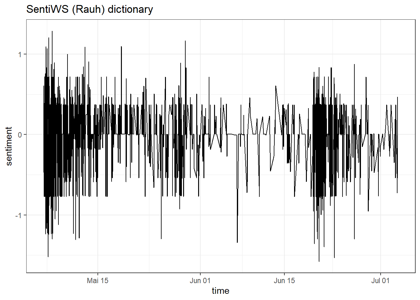

This graph looks as if the debate around Kliemann was polarized, i.e., that negative buzz also produced positive counterarguing (at least most of the time).

Task 8: Sentiment over time periods

Using the German SentiWS_Rauh dictionary, try to do a similar analysis with the Kliemann data and investigate the sentiment for each individual month starting and ending with the 6th day of this month. Our data from stretches from 6th of May to 3rd of July, so you have to include these three days of July in the June time period.

library(lubridate)

data_tknzd %>%
  inner_join(sentiWS) %>%
  mutate(period = case_when(
    time <= ymd_hms('2022-06-05 23:59:59') ~ "May",
    time >= ymd_hms('2022-06-06 00:00:00') ~ "June")) %>%
  mutate(sentiment = case_when(
    value < 0 ~ "negative",
    value > 0 ~ "positive"
  )) %>%
  count(period, sentiment)

## # A tibble: 4 × 3
##   period sentiment     n
##   <chr>  <chr>     <int>
## 1 June   negative   1077
## 2 June   positive   1789
## 3 May    negative   1732
## 4 May    positive   3979