1 Tutorial: Installing & Understanding R/R Studio

After working through Tutorial 1, you’ll…

know how to install R and R Studio
know how to update R and R Studio
understand the layout of R Studio

1.1 Installing R

R is the programming language we’ll use to import, edit, and analyze data. Please watch one of these two video tutorials before installing R yourself.

When you are ready to install R, use Cran to install the newest version of R (4.1.2, “Bird Hippie”). You’ll have to specify your operation system to download the right version:

1.2 Installing R Studio

Next, install R Studio. R Studio is a desktop application with a graphical interface that facilitates programming with R. The newest version of R Studio (1.4.1717) can be downloaded via this Link.

1.3 Updating R and R Studio

If you have already installed R and RStudio (for example, because you already needed it for a previous seminar), please update your version to the latest version. This way, we’ll all know that our versions are compatible.

1.3.1 On Windows

Updating on Windows is tricky. Therefore, you can use a package called installr, which helps you manage your update. First, install the installr package if you don’t have it. Use the following code:

# installing/loading the package:
if(!require(installr)) {
  install.packages("installr"); 
  require(installr)
} #load / install+load installr

After you have installed or loaded the installr package, let’s start the updating process of your R installation by using the updateR() function. It will check for newer versions, and if one is available, will guide you through the decisions you’d need to make:

# using the package:
updateR()

Finally, update R Studio. Updating RStudio is easy, just open RStudio and go to Help > Check for Updates to install a newer version.

1.3.2 On MAC

Go to CRAN and install the newer package installer.

After that update R Studio. Updating RStudio is easy, just open RStudio and go to Help > Check for Updates to install a newer version.

1.4 How does R work?

R is an object- and function-oriented programming language. Chambers (2014, p. 4) explains “object- and function-oriented” like this:

Everything that exists is an object.
Everything that happens is a function call.

IN R, you will assign values (for instance, single numbers/letters, several numbers/letters, or whole data files) to objects in R to work with them. For example, this command will assign the letters “hello” to an object caled word by using the assign operator <- (a function used to assign values to objects):

word <- "hello"

The type of each object will dictate what sorts of computations you may be done with this object. The object word, for example, is distinguished by the fact that it is made up of characters (i.e., it is a word) - which may make it impossible to compute the object’s mean value, for example (which is possible only for objects consisting of numerical data).

1.5 Why should I use R?

There are several reasons why I’m an advocate of R (or similar programming languages such as Python) over programs such as SPSS.

R is free. Other than most other (statistical) programs, you do not need to buy it (or rely on an university license, that is likely to run out once you leave your department).
R is an open source program. Other than most other programs, the source code - i.e., the basis of the program - is freely available. So are the hundred of packages (we’ll get to those later – these are basically additional functions you may need for more specific analyses) on CRAN that you can use to extend R’s base functions.
R offers you flexibility. You can work with almost any type of data and rely on a large (!) set of functions to import, edit, or analyze such data. And if the function you need to do so hasn’t been implemented (or simply does not exist yet), you can write it yourself!
Learning R increases your chances on the job market. For many jobs (academia, market research, data science, data journalism), applicants should know at least one programming language.

1.6 How does R Studio work?

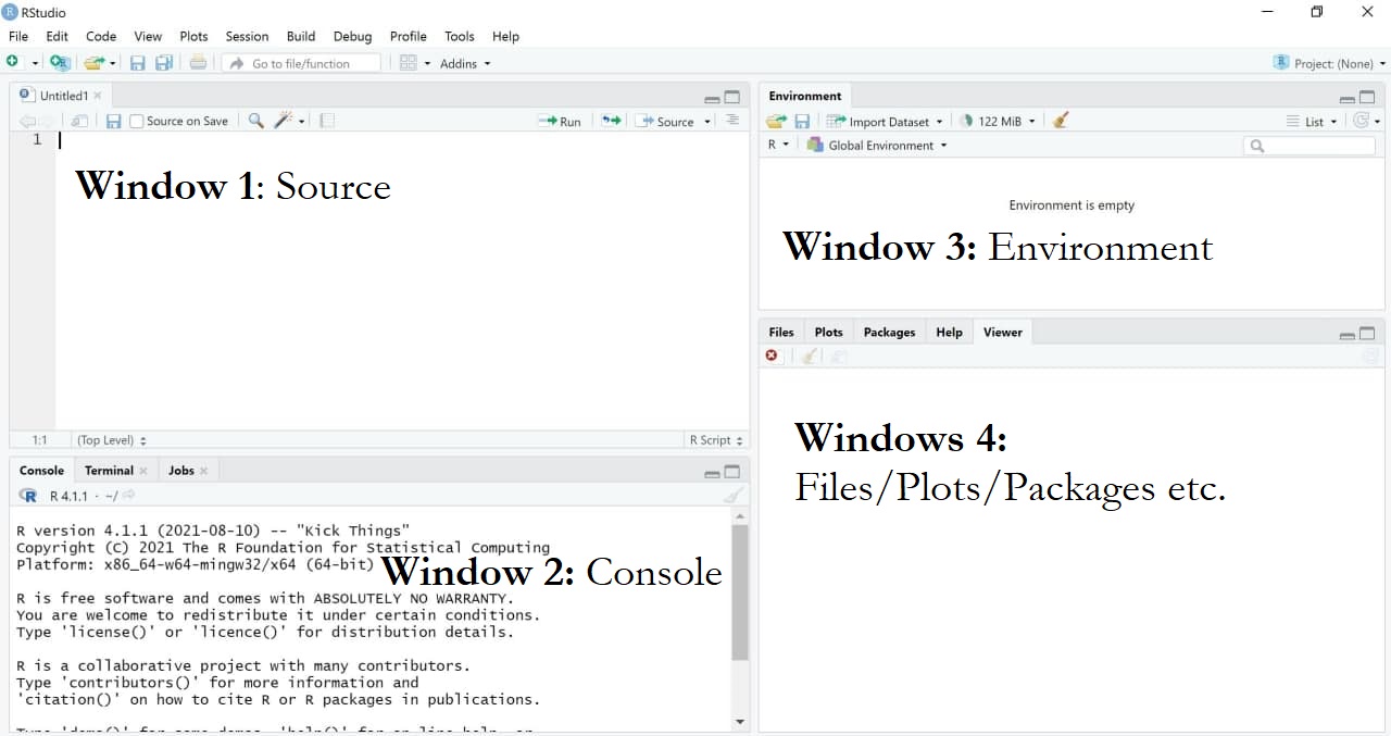
As mentioned, R studio is a graphical interface which facilitates programming with R. It contains up to four main windows, which allow for different things:

Writing your own code (Window 1: Source). Important: When first installing R/R Studio and opening R studio, you may not see this window right away. In this case, simply open it by clicking on File/New File/R Script.
Executing your own code (Window 2: Console)
Inspecting objects (Window 3: Environment)
Visualizing data, searching for help, updating packages etc. (Window 4: Files/Plots/Packages etc.)

Image: Four main windows in R

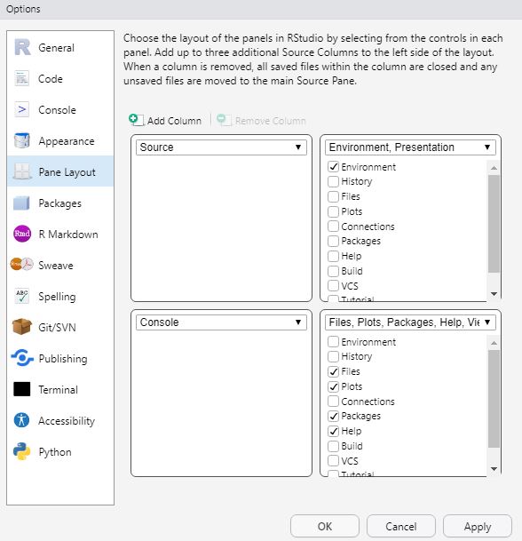
Please note that the specific set-up of your R Studio may look different (the order of windows may vary and so may the windows’ names). I have made the experience that having these four windows open works best for me. This may be different for you. If you want to modify the appearance of your R Studio, simply choose “Tools/Global Options/Pane Layout”.

Image: Changing the Layout

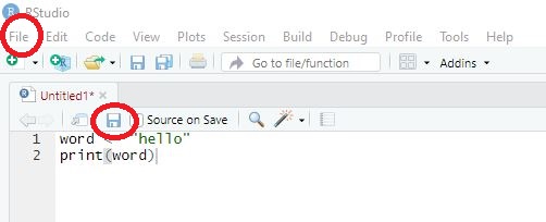
1.6.1 Source: Writing your own code

Using the window “Source”, you’ll write your own code to execute whichever task you want R to fulfill.

1.6.1.1 Writing Code

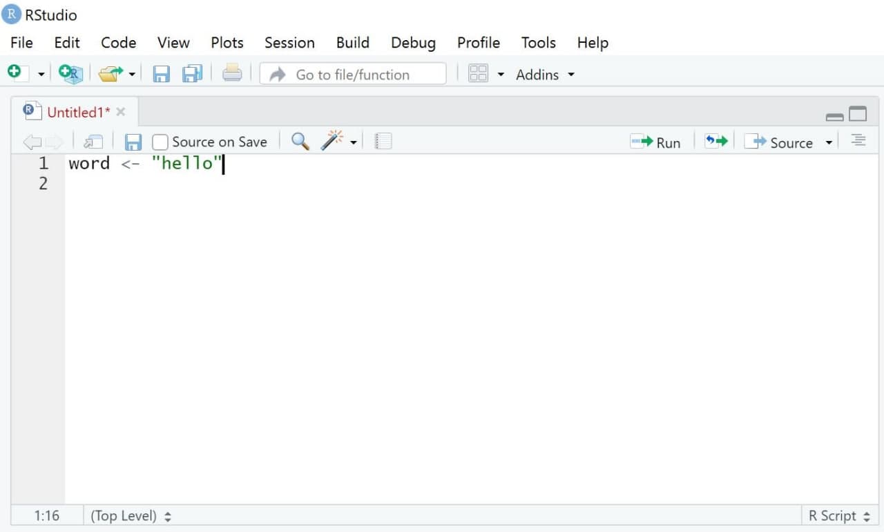
Let’s start with an easy example: Assume you simply want R to print the word “hello”. In this case, you would first write a simple command that assigns the word “hello” to an object called word. The assigment of values to named objects is done via either the operator “<-” or the operator “=”. The left side of that command contains the object that should be created; its right side the values that should be assigned to this object.

In short, this command tells R to assign the world “hello” to an object called word.

word <- "hello"

Image: “Source”

1.6.1.2 Annotating Code

Another helpful aspect of R is that you can comment your own code. Oftentimes, this is very helpful for understanding your code later (if you write several hundred lines of codes, you may not remember their exact meaning months later).

Comments or notes can be made via hashtags #. Anything following a hashtag will not be considered code by R but be ignored instead.

word <- "hello" #this line of code assigns the word "hello" to an object called word

1.6.1.3 Executing Code

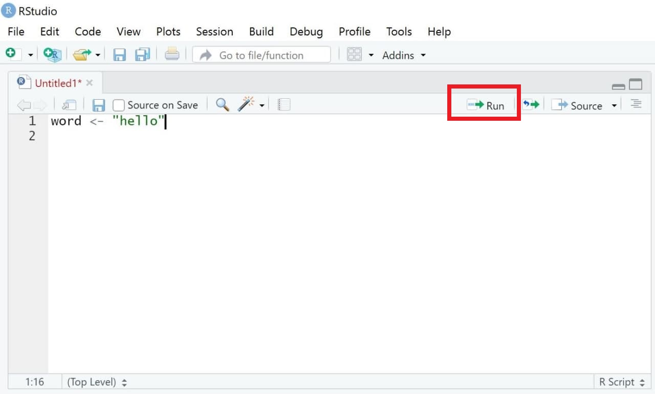
We now want to execute our code. Doing so is simple:

Mark the parts of the code you want to run (for instance, single rows of code or blocks of code across several rows)
Either press Run (see upper right side of the same window) or press Ctrl + Enter (On Mac OS X, hold the command key and press return instead).

R should now execute exactly those lines of codes that you marked (hereby creating the object word). If you haven’t marked any specific code, all lines of code will be executed.

Image: Executing Code

1.6.1.4 Saving Code

A great feature of R is that it makes analyses easily reproducible - given that you save your code. When reopening R Studio and you script, you can simply “rerun” the code with one click and your analysis will be reproduced.

To save code, you have two options:

Choose the menu option File/Save as. Important: Code needs to be saved with the ending “.R”.
Chose the Save-button in the source window and save your code in the correct format, for instance as “MyCode.R”.

Image: Saving code

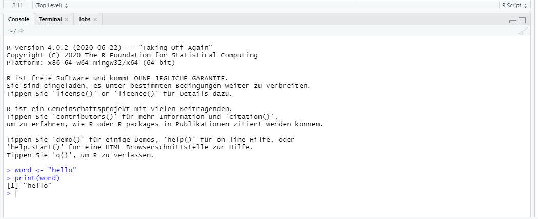
1.6.2 Console: Printing results

Results of executing code are printed in a second window called “Console”, which includes the code you ran and the object you may have called when doing so.

Previously, we defined an object called word, which consists of the single word “hello”. Thus, R prints our code as well as objects called when running this code (here, the object word) in the console.

word <- "hello"
word

## [1] "hello"

Image: Window “Console”

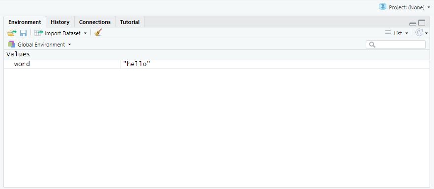
1.6.3 Environment: Overview of objects

The third window is called “Environment”¹. This windows displays all the objects currently existing - in our case, only the object “word”. As soon as you start creating more objects, this environment will fill up.

If you’re an SPSS user, this window is very similar to what is called the Datenansicht / Data overview in SPSS. However, the R version of this is much more flexible, given that our environment can contain several data sets, for example, at the same time.

Image: Window “Environment”

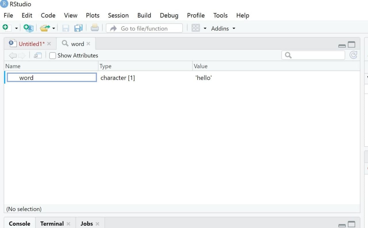
It is important to know that we can visually inspect any object using the View() command (with a new tab then opening in the “Source” window). This isn’t super helpful right now - but if you work with bigger data sets with several observations/variables later on, it is often useful to inspect data visually.

View(word)

Image: Window “View”

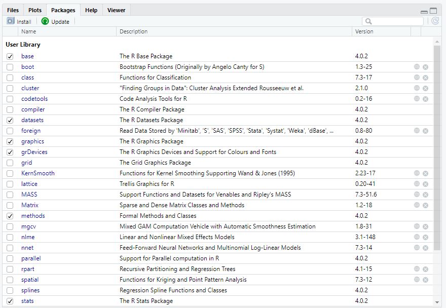
1.6.4 Plots/Help/Packages: Do everything else

Lastly, the standard R Studio interface contains a fourth window (if you opted for this layout). In my case, the window contains several sub-sections called “Files”, “Plots”, or “Packages” among others. You’ll understand their specific functions later - the window can, for instance, be used to plot/visualize results or see which packages are currently loaded.

Image: Window “Files/Plots/Packages”

1.7 Packages

While Base R, i.e., the standard version of R, already includes many helpful functions, you may at times need other, additional functions. For instance, if we want to perform text analysis in R we’ll need to use specific packages including additional functions.

Packages are collections of topic-specific functions that extend the functions implemented in Base R.

In the spirit of “open science”, anyone can write and publish these additional functions and related packages and anyone can also access the code used to do so.

You’ll find a list of all of R packages here. In this seminar, we’ll for instance use packages like dplyr for advanced data management.

1.7.1 Installing packages

To use a package, you have to install it first. Let’s say you’re interested in using the package dplyr. Using the command install.packages(), you can install the package on your computer. You’ll have to give the function the name of the package you are interested in installing.

install.packages("dplyr")

Now the package has been installed on your computer and is accessible locally. We only have to use install.packages() for any package once. Afterwards, the only thing you’ll have to do after open R is to activate the already installed package - which we’ll learn next.

1.7.2 Activating packages

Before we are able to use a package, we need to activate it in each session. Thus, you should not only define a working directory at the beginning of each session but also activate the packages you want to use via the library()_ command. Again, you’ll have to give R the name of the package you want to activate:

library(dplyr)

You can also use the name of the package followed by two colons :: to activate a package directly before calling one of its function. For instance, I do not need use to activate the dplyr package (by using the library() function) to use the function summarize() if I use the following code:

dplyr::summarize()

1.7.3 Getting information about packages

The package is installed and activated - but how can we use it? To get an overview of functions included in a given package, you can consult its corresponding “reference manual” (overview document containing all of a package’s functions) or, if available, its “vignette” (tutorials on how to use selected functions for the corresponding package) provided by a package’s author on a website called “CRAN”.

The easiest way to finding these manuals/vignettes is Google: Simply google CRAN ProcessR, for instance, and you’ll be guided to the following website:

Image: Cran Overview dplyr package

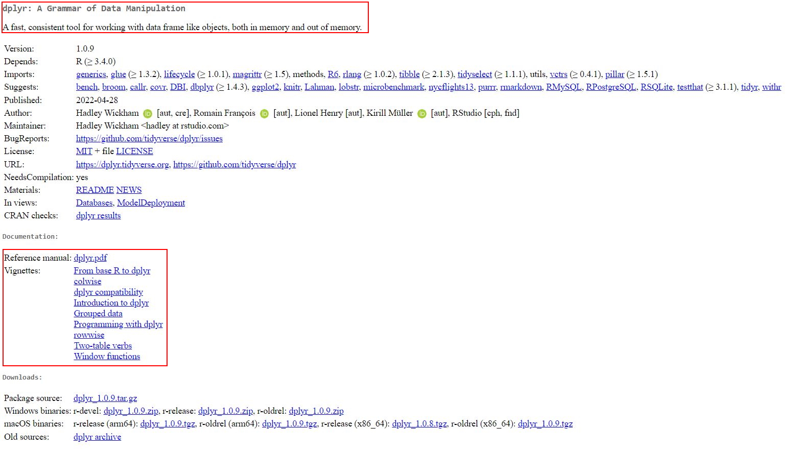The first paragraph (circled in red) gives you an overview of aspects for which this package may be useful. The second red-circled area links to the reference manual and the vignette. You can, for instance, check out the reference manual to get an idea of the many functions the dplyr package contains.

1.8 Take-Aways

Window “Source”: used to write/execute code in R
Window “Console”: used to return results of executed code
Window “Environment”: used to inspect objects on which to use functions
Window “Files/Plots/Packages etc.”: used for additional functions, for instance visualizations/searching for help/activating or updating packages

1.9 Additional tutorials

You still have questions? The following tutorials & papers can help you with that:

Now that you know the layout of R, we can get started with some real action: Tutorial: Using R as a calculator

again, this only applies for the way I set up my R Studio. You can change this via “Tools/Global Options/Pane Layout”↩︎