4 Tutorial: Data management with tidyverse

After working through Tutorial 4, you’ll…

• know the advantages of the tidyverse vs. Base R
• know about different formats of tabular data
• understand what packages are included in the tidyverse meta-package
• know how to do data modifications and transformations with dplyr

4.1 Why not stick with Base R?

You might wonder why we’ve spent so much time exploring functions in Base R to now learn data management with tidyverse. After all, data management can also be done in Base R, can’t it? I personally recommend that all R beginners should work with the tidyverse as early as possible. There are three reasons supporting my argument:

1. Ease of use: The tidyverse is very accessible for R “beginners”, i.e. its syntax is very easy to understand. It allows you to set goals (i.e. what you want to do with your data) and get you working on these goals very quickly. Definitely more quickly than in Base R!
2. Standard for data management: A few years ago, the tidyverse has become the de facto standard for data management in R. It is a meta-package, which means that it is a collection of distinct packages that all follow the same design principles to make code reading and writing as simple as possible. For example, all functions are named after verbs that indicate exactly what they perform (e.g. filter or summarize).
3. Beautiful graphs: With the tidyverse, all data management steps can be swiftly transferred into beautiful graphs. This is because the most popular graph package in R, ggplot2, is part of the tidyverse.

Are you excited now? Then let’s get started!

4.2 Tidyverse packages

The tidyverse comes with a great arsenal of topic-specific packages and their respective functions. It includes packages for:

• tibble: creating data structures like tibbles, which is an enhanced type of data frame
• readr, haven, readxl: reading data (e.g. readr for CSV, haven for SPSS, Stata and SAS, readxl for Excel)
• tidyr, dplyr: data transformation, modification, and summary statistics
• stringr, forcats, lubridate: create special, powerful object types (e.g. stringr for working with text objects, forcats for factors, lubridate for time data)
• purrr: programming with R
• ggplot2: graphing/charting

The most frequently used packages of the tidyverse can be installed and activated in one go (less frequently used packages like haven still need to be installed and activated separately):

install.packages("tidyverse") # install the package (only on the first time)
library(tidyverse) # active the package

4.3 Tidy data

Dataframes, which we learned about in [Types of objects], are tabular data. However, data can also have other formats, for example as nested, i.e. hierarchical, lists. In communication research, these other data formats are mainly used by social media and their respective APIs (perhaps you have heard of the “JSON” format before).

In our course, however, we’ll focus on tabular data.The same data can be represented differently in tables. We perceive some of these representations as tidy, others as messy. While tidy data principles establish a standard for organizing data values inside a data frame and thus all tidy data look the same, every messy dataset is messy in its own way.

Take a look at the table below. It shows a Starwars data set that comes pre-installed with the dplyr package. Do you feel the tabled data is messy? Why (not)?

## # A tibble: 10 × 3
##    name                  body_feature value
##    <chr>                 <chr>        <dbl>
##  1 Anakin Skywalker      height         188
##  2 Anakin Skywalker      mass            84
##  3 Chewbacca             height         228
##  4 Chewbacca             mass           112
##  5 Darth Vader           height         202
##  6 Darth Vader           mass           136
##  7 Jabba Desilijic Tiure height         175
##  8 Jabba Desilijic Tiure mass          1358
##  9 Leia Organa           height         150
## 10 Leia Organa           mass            49

Overall, this data is messy. It comes with three messy problems:

1. This body_feature column comprises information relating to both height and weight, i.e. both variables are stored in a single column.
2. As a result, the value column is reliant on the body_feature column; we can’t tell the stored values apart by merely looking at the value column. We always need to check the body_feature column.
3. Consequently, we have issues with vectorized functions (remember, in R, columns in data sets are vectors): We can’t, for example, use the mean() function on the value column to determine the average weight of the Star Wars characters since the height values are also stored there.

What do you think of this table? Is it messy?

## # A tibble: 5 × 3
##   name                  height  mass
##   <chr>                  <int> <dbl>
## 1 Anakin Skywalker         188    84
## 2 Chewbacca                228   112
## 3 Darth Vader              202   136
## 4 Jabba Desilijic Tiure    175  1358
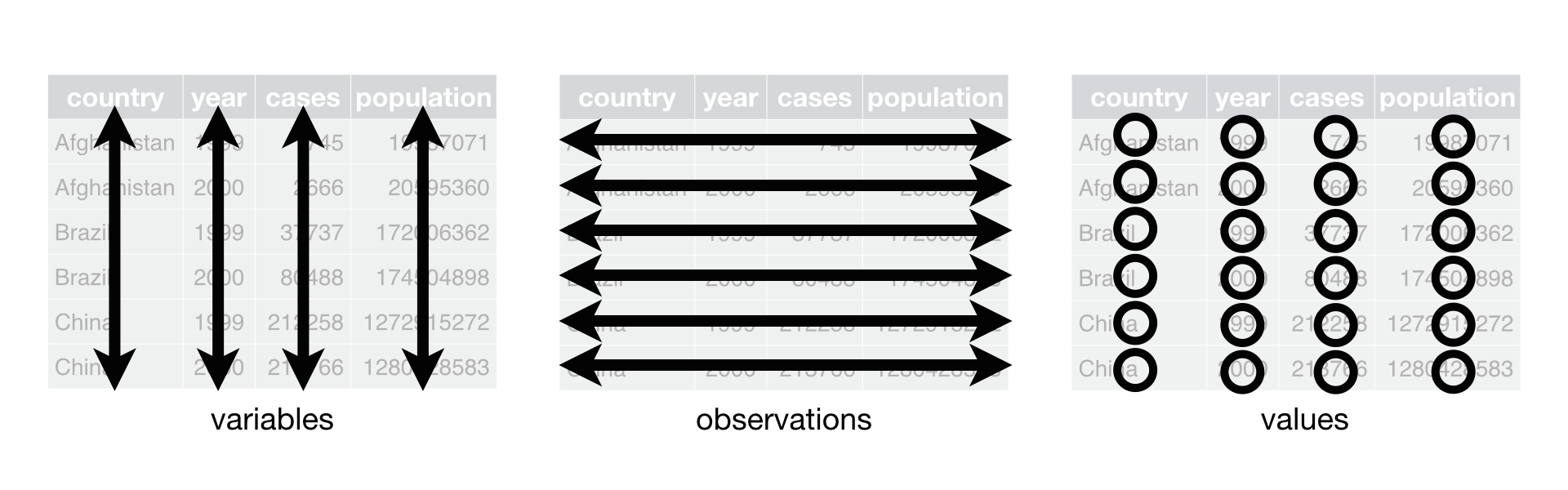
## 5 Leia Organa              150    49

This table looks tidy! Tidy data is a standard way of mapping the meaning of a dataset to its structure. We determine whether a dataset is messy or tidy depending on how rows, columns and tables are matched up with observations, variables and types. We consider a table tidy when it follows the following golden rules:

1. Columns: Every column is one variable.
2. Rows: Every row is one observation.
3. Cells: Every cell contains one single value.

Image: The tidy data principle (Source: R for Data Science)

In messy data sets, on the other hand…

1. Column headers are values, not variable names.
2. Multiple variables are stored in one column.
3. Variables are stored in both rows and columns.
4. Multiple types of observational units are stored in the same table.
5. A single observational unit is stored in multiple tables.

Why should you be concerned about tidy data organization?

There are two major advantages:

1. When you have a consistent data structure, it is easier to learn the respective tools that work well with this data structure. dplyr, ggplot2, and all the other tidyverse packages are designed for working with tidy data.
2. Putting variables in columns makes R’s vectorized nature shine. The majority of built-in R-functions (like the mean() function) works with vectors of values. As a result, the tidy reorganization of data seems only natural for a good work flow in R.

If you have been working mainly with survey data, then you will already be familiar with these basic rules, as data export from survey software usually follows these principles. However, “real-world” data from databases or social media often does not follow these principles. That’s why it’s sometimes true to say that 80% of data analysis is spent on cleaning and transforming data.

4.4 The pipe operator

Truly, dplyr is my favorite tidyverse package (even more so than ggplot2, which we’ll cover later!). It allows you to perform powerful data transformations in just a few simple steps.

To this end, dplyr relies on the pipe operator (%>%).² The %>% operator allows functions to be applied sequentially to the same source object in a concise manner, so that step-by-step transformations can be applied to the data. Therefore, we always call the source object first and then add each transformation step separated by the %>% operator. Let’s illustrate this concept with an example. We’ll use the Starwars data set that you are already familiar with.

starwars_data %>%    # First, we define the source object, i.e. the data frame that we want to transform, followed by the pipe operator 
  plot()             # Second, we specify which function should be performed on the source object, here: scatterplot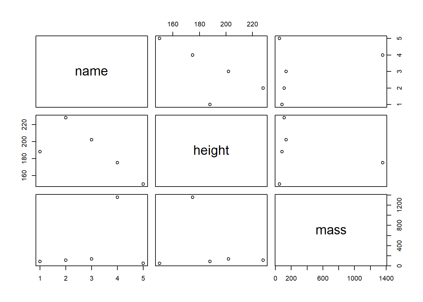

Now, that’s not very impressive. We could do the same in Base R like this:

plot(starwars_data)

However, dplyr gets really impressive when you chain functions sequentially. You can apply certain selection criteria to your data and plot it in one go. For example, we might exclude the variable name from our scatter plot, since it’s not a metric variable anyway. Also, we might want to look only at those Star Wars characters taller than 170 cm. Let’s try it in a single run!

starwars_data %>%              # Define the source object
  select(height, mass) %>%     # Keep only the height and mass column
  filter(height > 170) %>%     # Filter all observations that are taller than 170cm  
  plot()                       # Plot!

Now try to do the same in Base R:

plot(starwars_data[starwars_data$height>170,]$mass~starwars_data[starwars_data$height>170,]$height, xlab="height", ylab="mass")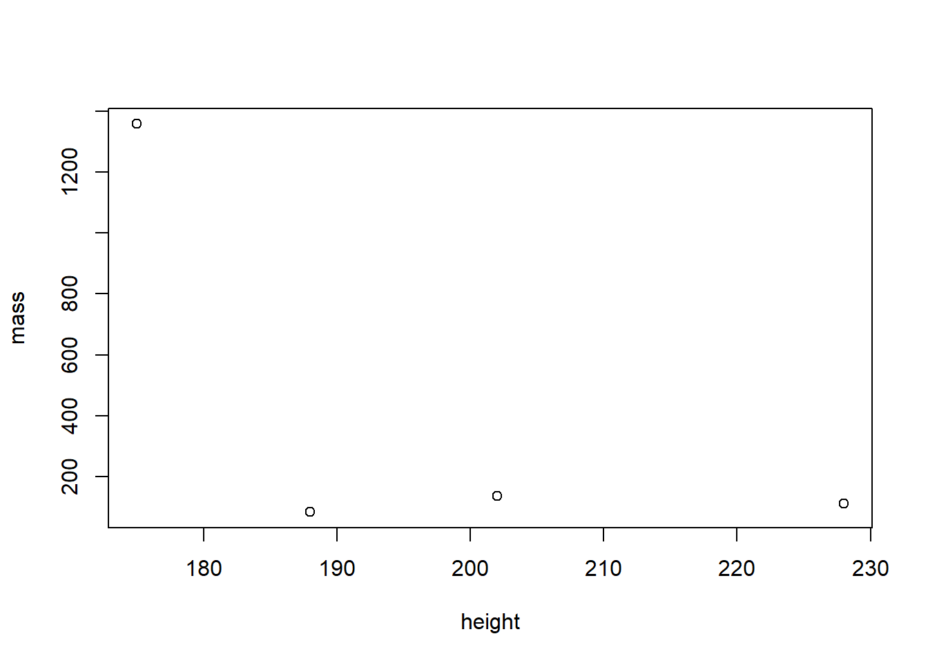

The Base R code is longer, more nested, and not as readable as the code written in dplyr. And the more selection criteria and functions you need to implement, the worse it gets. For example, imagine you would also want to exclude Star Wars characters with a mass bigger than 1200kg. Peace of cake with dplyr:

starwars_data %>%              
  select(height, mass) %>%     
  filter(height > 170) %>%
  filter(mass < 1200) %>% 
  plot()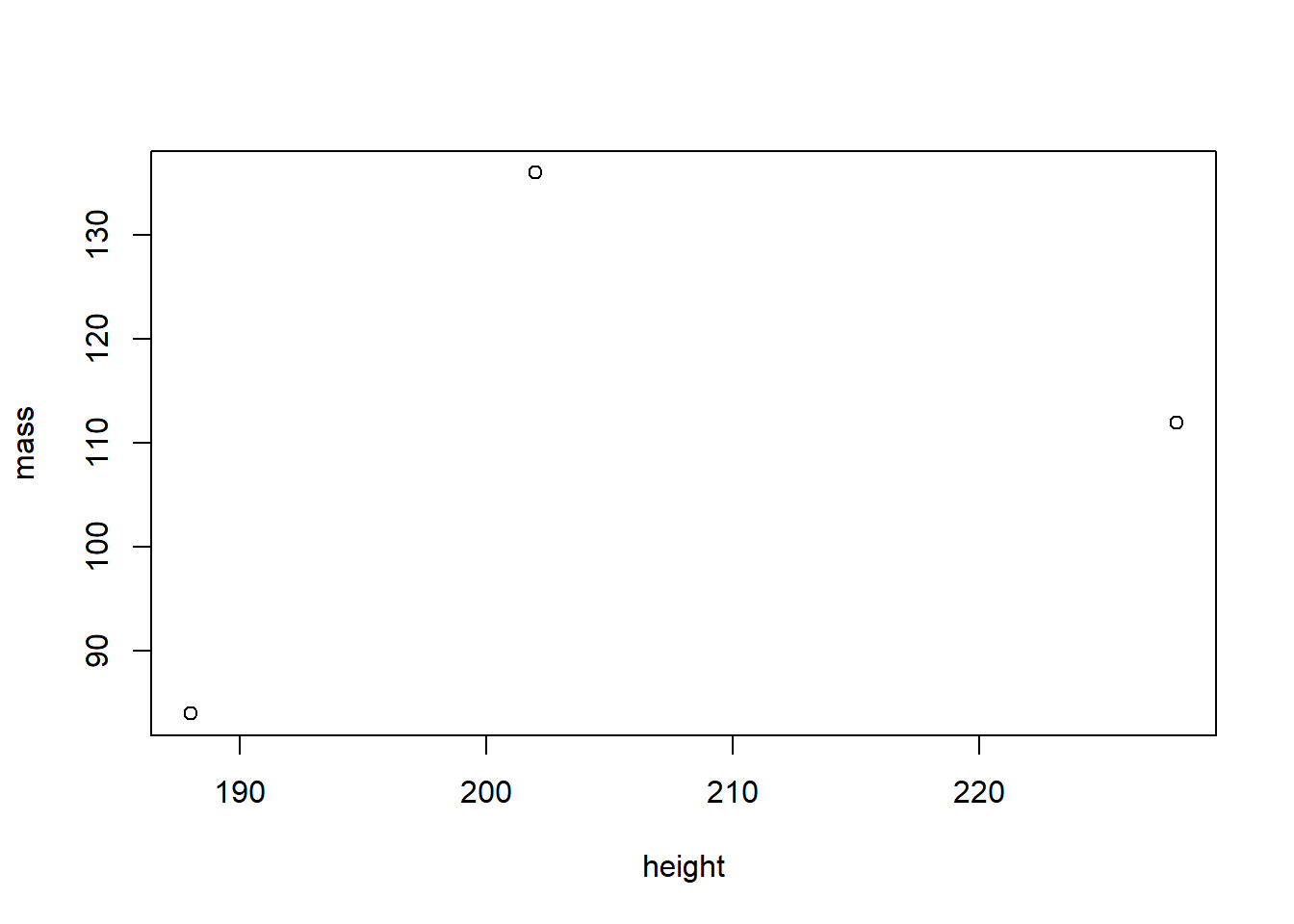                       

4.5 Data transformation with dplyr

dplyrcomes with five main functions:

1. select(): select variables column by column, i.e. pick columns / variables by their names
2. filter(): filter observations row by row, i.e. pick observations by their values
3. arrange(): sort / reorder data in ascending or descending order
4. mutate(): calculate new variables or transform existing ones
5. summarize(): summarize variables (e.g. mean, standard deviation, etc.), best combined with group_by()

4.5.1 select()

Scientists will frequently provide you with large data sets including hundreds of variables (often even more!). The first problem in this scenario is narrowing down the variables you are truly interested in. select() helps you to easily choose a suitable subset of variables. In this selection process, the name of the data frame is the source object, followed by the pipe %>% operator. The expression that selects the columns that you are interested in comes after that.

Take the Star Wars data, for example. The original data set has 87 observations (Star Wars characters) and 14 columns / variables (traits of these characters, e.g., birth_year, gender, and species). Yes, 14 columns is not a lot and you could get an overview of this data without subsetting columns. Let’s take a look at the original data frame:

library(dplyr)            # load dplyr
starwars_data <- starwars # assign the pre-installed starwars data from dplyr to a source object / variable

starwars_data             # print the content of the data frame to the console

## # A tibble: 87 × 14
##    name     height  mass hair_color skin_color eye_color birth_year sex   gender
##    <chr>     <int> <dbl> <chr>      <chr>      <chr>          <dbl> <chr> <chr> 
##  1 Luke Sk…    172    77 blond      fair       blue            19   male  mascu…
##  2 C-3PO       167    75 <NA>       gold       yellow         112   none  mascu…
##  3 R2-D2        96    32 <NA>       white, bl… red             33   none  mascu…
##  4 Darth V…    202   136 none       white      yellow          41.9 male  mascu…
##  5 Leia Or…    150    49 brown      light      brown           19   fema… femin…
##  6 Owen La…    178   120 brown, gr… light      blue            52   male  mascu…
##  7 Beru Wh…    165    75 brown      light      blue            47   fema… femin…
##  8 R5-D4        97    32 <NA>       white, red red             NA   none  mascu…
##  9 Biggs D…    183    84 black      light      brown           24   male  mascu…
## 10 Obi-Wan…    182    77 auburn, w… fair       blue-gray       57   male  mascu…
## # … with 77 more rows, and 5 more variables: homeworld <chr>, species <chr>,
## #   films <list>, vehicles <list>, starships <list>

For the sake of practice, let’s say we only want to analyze the species, birth_year, mass, and height of these characters. To simplify data handling, we want to keep only the respective columns.

starwars_data %>%                                 # define the source object
  select(name, species, birth_year, mass, height) # keep only the name, species, birth_year, mass and height column

## # A tibble: 87 × 5
##    name               species birth_year  mass height
##    <chr>              <chr>        <dbl> <dbl>  <int>
##  1 Luke Skywalker     Human         19      77    172
##  2 C-3PO              Droid        112      75    167
##  3 R2-D2              Droid         33      32     96
##  4 Darth Vader        Human         41.9   136    202
##  5 Leia Organa        Human         19      49    150
##  6 Owen Lars          Human         52     120    178
##  7 Beru Whitesun lars Human         47      75    165
##  8 R5-D4              Droid         NA      32     97
##  9 Biggs Darklighter  Human         24      84    183
## 10 Obi-Wan Kenobi     Human         57      77    182
## # … with 77 more rows

At the moment you have only printed the transformed data to the console. However, most of the time we want to keep the transformed data ready for further calculations. In this case we should assign the transformed data into a new source object, which we can access later.

starwars_short <- starwars_data %>%                   # assign a new source object and define the old source object
  select(name, species, birth_year, mass, height)     # keep only the name, species, birth_year, mass and height column

Let’s print the new source object, starwars_short, to the console.

starwars_short

## # A tibble: 87 × 5
##    name               species birth_year  mass height
##    <chr>              <chr>        <dbl> <dbl>  <int>
##  1 Luke Skywalker     Human         19      77    172
##  2 C-3PO              Droid        112      75    167
##  3 R2-D2              Droid         33      32     96
##  4 Darth Vader        Human         41.9   136    202
##  5 Leia Organa        Human         19      49    150
##  6 Owen Lars          Human         52     120    178
##  7 Beru Whitesun lars Human         47      75    165
##  8 R5-D4              Droid         NA      32     97
##  9 Biggs Darklighter  Human         24      84    183
## 10 Obi-Wan Kenobi     Human         57      77    182
## # … with 77 more rows

You can also delete columns by making a reverse selection with the - symbol. This means that you select all columns except the one whose name you specify.

starwars_short %>%                     
  select(-name)                      # keep all columns except the name column (i.e. delete name column)

## # A tibble: 87 × 4
##    species birth_year  mass height
##    <chr>        <dbl> <dbl>  <int>
##  1 Human         19      77    172
##  2 Droid        112      75    167
##  3 Droid         33      32     96
##  4 Human         41.9   136    202
##  5 Human         19      49    150
##  6 Human         52     120    178
##  7 Human         47      75    165
##  8 Droid         NA      32     97
##  9 Human         24      84    183
## 10 Human         57      77    182
## # … with 77 more rows

You can delete more than one column in one go:

starwars_short %>%                     
  select(-c(name,species))           # keep all columns except the name & species column (i.e. delete these columns)

## # A tibble: 87 × 3
##    birth_year  mass height
##         <dbl> <dbl>  <int>
##  1       19      77    172
##  2      112      75    167
##  3       33      32     96
##  4       41.9   136    202
##  5       19      49    150
##  6       52     120    178
##  7       47      75    165
##  8       NA      32     97
##  9       24      84    183
## 10       57      77    182
## # … with 77 more rows

Tip for advanced users: You can select columns and rename them at the same time.

starwars_short %>%                     
  select("character"=name, "age"=birth_year)      # select columns that you want to keep & rename them

## # A tibble: 87 × 2
##    character            age
##    <chr>              <dbl>
##  1 Luke Skywalker      19  
##  2 C-3PO              112  
##  3 R2-D2               33  
##  4 Darth Vader         41.9
##  5 Leia Organa         19  
##  6 Owen Lars           52  
##  7 Beru Whitesun lars  47  
##  8 R5-D4               NA  
##  9 Biggs Darklighter   24  
## 10 Obi-Wan Kenobi      57  
## # … with 77 more rows

4.5.2 filter()

filter() divides observations into groups depending on their values. The name of the data frame is the source object, followed by the pipe %>% operator. Then follow the expressions that filter the data.

Let’s only select human Star Wars characters in our transformed data set starwars_short:

starwars_short %>%
  filter(species=="Human")

## # A tibble: 35 × 5
##    name               species birth_year  mass height
##    <chr>              <chr>        <dbl> <dbl>  <int>
##  1 Luke Skywalker     Human         19      77    172
##  2 Darth Vader        Human         41.9   136    202
##  3 Leia Organa        Human         19      49    150
##  4 Owen Lars          Human         52     120    178
##  5 Beru Whitesun lars Human         47      75    165
##  6 Biggs Darklighter  Human         24      84    183
##  7 Obi-Wan Kenobi     Human         57      77    182
##  8 Anakin Skywalker   Human         41.9    84    188
##  9 Wilhuff Tarkin     Human         64      NA    180
## 10 Han Solo           Human         29      80    180
## # … with 25 more rows

And now let’s only select Star Wars character who are younger than 24 or exactly 24 years old.

starwars_short %>%
  filter(birth_year<=24)

## # A tibble: 7 × 5
##   name                  species birth_year  mass height
##   <chr>                 <chr>        <dbl> <dbl>  <int>
## 1 Luke Skywalker        Human           19    77    172
## 2 Leia Organa           Human           19    49    150
## 3 Biggs Darklighter     Human           24    84    183
## 4 Wedge Antilles        Human           21    77    170
## 5 IG-88                 Droid           15   140    200
## 6 Wicket Systri Warrick Ewok             8    20     88
## 7 Plo Koon              Kel Dor         22    80    188

Chaining some functions, let’s look at Star Wars character who are a Droid and older than 24.

starwars_short %>%
  filter(species=="Droid" & birth_year > 24)   # & --> filter all observations to which both logical statements apply

## # A tibble: 2 × 5
##   name  species birth_year  mass height
##   <chr> <chr>        <dbl> <dbl>  <int>
## 1 C-3PO Droid          112    75    167
## 2 R2-D2 Droid           33    32     96

Alternatively, you can also write these filters like this:

starwars_short %>%
  filter(species=="Droid") %>%
  filter(birth_year > 24)

## # A tibble: 2 × 5
##   name  species birth_year  mass height
##   <chr> <chr>        <dbl> <dbl>  <int>
## 1 C-3PO Droid          112    75    167
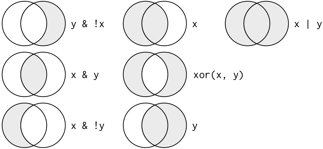
## 2 R2-D2 Droid           33    32     96

Besides the & operator, there are many more logical operators that you can choose from to optimize your filter choices. Here is an overview:

Image: Logical, i.e. boolean, operators (Source: R for Data Science)

Tip for advanced users 1: You can negate filters. This means that you keep all observations except the one that you have specified with the != operator (read != as: is not or is unequal to). For example, you can choose to include only non-human Star Wars characters.

starwars_short %>%
  filter(species!="Human")

## # A tibble: 48 × 5
##    name                  species        birth_year  mass height
##    <chr>                 <chr>               <dbl> <dbl>  <int>
##  1 C-3PO                 Droid                 112    75    167
##  2 R2-D2                 Droid                  33    32     96
##  3 R5-D4                 Droid                  NA    32     97
##  4 Chewbacca             Wookiee               200   112    228
##  5 Greedo                Rodian                 44    74    173
##  6 Jabba Desilijic Tiure Hutt                  600  1358    175
##  7 Yoda                  Yoda's species        896    17     66
##  8 IG-88                 Droid                  15   140    200
##  9 Bossk                 Trandoshan             53   113    190
## 10 Ackbar                Mon Calamari           41    83    180
## # … with 38 more rows

Alternatively, you achieve the same goal by negating the entire function call. Negating the entire function call can be handy at times.

starwars_short %>%
  filter(!(species=="Human"))

## # A tibble: 48 × 5
##    name                  species        birth_year  mass height
##    <chr>                 <chr>               <dbl> <dbl>  <int>
##  1 C-3PO                 Droid                 112    75    167
##  2 R2-D2                 Droid                  33    32     96
##  3 R5-D4                 Droid                  NA    32     97
##  4 Chewbacca             Wookiee               200   112    228
##  5 Greedo                Rodian                 44    74    173
##  6 Jabba Desilijic Tiure Hutt                  600  1358    175
##  7 Yoda                  Yoda's species        896    17     66
##  8 IG-88                 Droid                  15   140    200
##  9 Bossk                 Trandoshan             53   113    190
## 10 Ackbar                Mon Calamari           41    83    180
## # … with 38 more rows

Tip for advanced users 2: You can filter for missing values (NAs) with the is.na() function.

starwars_short %>%
  filter(is.na(birth_year))

## # A tibble: 44 × 5
##    name             species   birth_year  mass height
##    <chr>            <chr>          <dbl> <dbl>  <int>
##  1 R5-D4            Droid             NA    32     97
##  2 Jek Tono Porkins Human             NA   110    180
##  3 Arvel Crynyd     Human             NA    NA     NA
##  4 Nien Nunb        Sullustan         NA    68    160
##  5 Nute Gunray      Neimodian         NA    90    191
##  6 Roos Tarpals     Gungan            NA    82    224
##  7 Rugor Nass       Gungan            NA    NA    206
##  8 Ric Olié         <NA>              NA    NA    183
##  9 Watto            Toydarian         NA    NA    137
## 10 Sebulba          Dug               NA    40    112
## # … with 34 more rows

And you can negate that filter to get rid of all observation that have missing values (NAs).

starwars_short %>%
  filter(!is.na(birth_year))

## # A tibble: 43 × 5
##    name               species birth_year  mass height
##    <chr>              <chr>        <dbl> <dbl>  <int>
##  1 Luke Skywalker     Human         19      77    172
##  2 C-3PO              Droid        112      75    167
##  3 R2-D2              Droid         33      32     96
##  4 Darth Vader        Human         41.9   136    202
##  5 Leia Organa        Human         19      49    150
##  6 Owen Lars          Human         52     120    178
##  7 Beru Whitesun lars Human         47      75    165
##  8 Biggs Darklighter  Human         24      84    183
##  9 Obi-Wan Kenobi     Human         57      77    182
## 10 Anakin Skywalker   Human         41.9    84    188
## # … with 33 more rows

Tip for advanced users 3: Watch out for the | operator (read: or). This one can be tricky to negate!

For example, with this code you get all characters that are NEITHER human NOR older than 33 years. I.e. you get all non-human characters who are younger than 33 or exactly 33 years old.

starwars_short %>%
  filter(!((species == "Human") | (birth_year > 33)))

## # A tibble: 4 × 5
##   name                  species birth_year  mass height
##   <chr>                 <chr>        <dbl> <dbl>  <int>
## 1 R2-D2                 Droid           33    32     96
## 2 IG-88                 Droid           15   140    200
## 3 Wicket Systri Warrick Ewok             8    20     88
## 4 Plo Koon              Kel Dor         22    80    188

But with this code, you’ll get all observations that are either non-human (regardless of their age) OR humans who are older than 33 years old.

starwars_short %>%
  filter((species != "Human") | (birth_year > 33))

## # A tibble: 67 × 5
##    name               species birth_year  mass height
##    <chr>              <chr>        <dbl> <dbl>  <int>
##  1 C-3PO              Droid        112      75    167
##  2 R2-D2              Droid         33      32     96
##  3 Darth Vader        Human         41.9   136    202
##  4 Owen Lars          Human         52     120    178
##  5 Beru Whitesun lars Human         47      75    165
##  6 R5-D4              Droid         NA      32     97
##  7 Obi-Wan Kenobi     Human         57      77    182
##  8 Anakin Skywalker   Human         41.9    84    188
##  9 Wilhuff Tarkin     Human         64      NA    180
## 10 Chewbacca          Wookiee      200     112    228
## # … with 57 more rows

4.5.3 arrange()

arrange() and filter() are like two brothers: both look similar, but they also differ in at least one essential aspect. Both functions change the rows of the data frame, but unlike filter(), arrange() does not select or delete rows, it only changes their order (either ascending or descending). By default, arrange() will sort in ascending order, i.e. from 1:100 (numeric vector) and from A:Z (character vector). arrange() must always be applied to at least one column that is to be sorted.

starwars_short %>%
  arrange(birth_year)

## # A tibble: 87 × 5
##    name                  species birth_year  mass height
##    <chr>                 <chr>        <dbl> <dbl>  <int>
##  1 Wicket Systri Warrick Ewok           8    20       88
##  2 IG-88                 Droid         15   140      200
##  3 Luke Skywalker        Human         19    77      172
##  4 Leia Organa           Human         19    49      150
##  5 Wedge Antilles        Human         21    77      170
##  6 Plo Koon              Kel Dor       22    80      188
##  7 Biggs Darklighter     Human         24    84      183
##  8 Han Solo              Human         29    80      180
##  9 Lando Calrissian      Human         31    79      177
## 10 Boba Fett             Human         31.5  78.2    183
## # … with 77 more rows

To get a descending order:

starwars_short %>%
  arrange(desc(birth_year))

## # A tibble: 87 × 5
##    name                  species        birth_year  mass height
##    <chr>                 <chr>               <dbl> <dbl>  <int>
##  1 Yoda                  Yoda's species        896    17     66
##  2 Jabba Desilijic Tiure Hutt                  600  1358    175
##  3 Chewbacca             Wookiee               200   112    228
##  4 C-3PO                 Droid                 112    75    167
##  5 Dooku                 Human                 102    80    193
##  6 Qui-Gon Jinn          Human                  92    89    193
##  7 Ki-Adi-Mundi          Cerean                 92    82    198
##  8 Finis Valorum         Human                  91    NA    170
##  9 Palpatine             Human                  82    75    170
## 10 Cliegg Lars           Human                  82    NA    183
## # … with 77 more rows

If you specify more than one column, then subsequent columns are used to break ties. Also note that missing values are always displayed last:

starwars_short %>%
  arrange(species, birth_year)

## # A tibble: 87 × 5
##    name            species  birth_year  mass height
##    <chr>           <chr>         <dbl> <dbl>  <int>
##  1 Ratts Tyerell   Aleena           NA    15     79
##  2 Dexter Jettster Besalisk         NA   102    198
##  3 Ki-Adi-Mundi    Cerean           92    82    198
##  4 Mas Amedda      Chagrian         NA    NA    196
##  5 Zam Wesell      Clawdite         NA    55    168
##  6 IG-88           Droid            15   140    200
##  7 R2-D2           Droid            33    32     96
##  8 C-3PO           Droid           112    75    167
##  9 R5-D4           Droid            NA    32     97
## 10 R4-P17          Droid            NA    NA     96
## # … with 77 more rows

4.5.4 mutate()

Often you want to add new columns to a data set, e.g. when you calculate new variables or when you want to store re-coded values of other variables. With mutate(), new columns will be added to the end of you data frame.

For example, we can resize the height column to provide the body height in m instead of cm. Let’s call that variable m_height. We’ll assign our transformed data (with the newly created m_height column) back into our source object (starwars_short) to keep the changes for the future (and not just print it to the console).

starwars_short <- starwars_short %>%     # assigns your source object, i.e. data, back to itself to save changes
  mutate(m_height=height/100)            # creates the new variable "m_height" and adds it to the end of the data frame

starwars_short                           # print the data to your console to inspect the new column

## # A tibble: 87 × 6
##    name               species birth_year  mass height m_height
##    <chr>              <chr>        <dbl> <dbl>  <int>    <dbl>
##  1 Luke Skywalker     Human         19      77    172     1.72
##  2 C-3PO              Droid        112      75    167     1.67
##  3 R2-D2              Droid         33      32     96     0.96
##  4 Darth Vader        Human         41.9   136    202     2.02
##  5 Leia Organa        Human         19      49    150     1.5 
##  6 Owen Lars          Human         52     120    178     1.78
##  7 Beru Whitesun lars Human         47      75    165     1.65
##  8 R5-D4              Droid         NA      32     97     0.97
##  9 Biggs Darklighter  Human         24      84    183     1.83
## 10 Obi-Wan Kenobi     Human         57      77    182     1.82
## # … with 77 more rows

Let’s calculate the BMI of the Star Wars characters with the BMI formula and the newly created m_height variable. Save the changes to your data frame by assigning the source object back to itself.

starwars_short <- starwars_short %>%     # assigns your source object, i.e. data, back to itself to save changes
  mutate(BMI= mass/m_height^2)           # creates the new variable "BMI" and adds it to the end of the data frame

starwars_short                           # print the data to your console to inspect the new column

## # A tibble: 87 × 7
##    name               species birth_year  mass height m_height   BMI
##    <chr>              <chr>        <dbl> <dbl>  <int>    <dbl> <dbl>
##  1 Luke Skywalker     Human         19      77    172     1.72  26.0
##  2 C-3PO              Droid        112      75    167     1.67  26.9
##  3 R2-D2              Droid         33      32     96     0.96  34.7
##  4 Darth Vader        Human         41.9   136    202     2.02  33.3
##  5 Leia Organa        Human         19      49    150     1.5   21.8
##  6 Owen Lars          Human         52     120    178     1.78  37.9
##  7 Beru Whitesun lars Human         47      75    165     1.65  27.5
##  8 R5-D4              Droid         NA      32     97     0.97  34.0
##  9 Biggs Darklighter  Human         24      84    183     1.83  25.1
## 10 Obi-Wan Kenobi     Human         57      77    182     1.82  23.2
## # … with 77 more rows

mutate() does not merely work with mathematical operators. You can also categorize numeric variables with the case_when function, which is part of the mutate() function.

starwars_short <- starwars_short %>%
  mutate(age_cat= case_when(            # "cat" is short for "categorized"
    birth_year < 20 ~ "very young",
    birth_year < 40 ~ "young",
    birth_year < 70 ~ "mid-aged",
    birth_year <= 100 ~ "old",
    birth_year > 100 ~ "very old")
    )

starwars_short

## # A tibble: 87 × 8
##    name               species birth_year  mass height m_height   BMI age_cat   
##    <chr>              <chr>        <dbl> <dbl>  <int>    <dbl> <dbl> <chr>     
##  1 Luke Skywalker     Human         19      77    172     1.72  26.0 very young
##  2 C-3PO              Droid        112      75    167     1.67  26.9 very old  
##  3 R2-D2              Droid         33      32     96     0.96  34.7 young     
##  4 Darth Vader        Human         41.9   136    202     2.02  33.3 mid-aged  
##  5 Leia Organa        Human         19      49    150     1.5   21.8 very young
##  6 Owen Lars          Human         52     120    178     1.78  37.9 mid-aged  
##  7 Beru Whitesun lars Human         47      75    165     1.65  27.5 mid-aged  
##  8 R5-D4              Droid         NA      32     97     0.97  34.0 <NA>      
##  9 Biggs Darklighter  Human         24      84    183     1.83  25.1 young     
## 10 Obi-Wan Kenobi     Human         57      77    182     1.82  23.2 mid-aged  
## # … with 77 more rows

Finally, you can recode variables by using the recode() function, which is part of the mutate() function. Let’s be crazy and recode all droids as robots³ and save the result in a new variable called crazy_species! Please note that recode() has an unusual syntax because it follows the order of old_var = new_var instead of the usual order: new_var = old_var. Therefore, recode() is likely to be retired in the future (use case_when instead).

starwars_short <- starwars_short %>% 
  mutate(crazy_species=recode( # alternatively, you could also recode directly back into the species variable
    species, "Droid"="Robot"))

starwars_short

## # A tibble: 87 × 9
##    name     species birth_year  mass height m_height   BMI age_cat crazy_species
##    <chr>    <chr>        <dbl> <dbl>  <int>    <dbl> <dbl> <chr>   <chr>        
##  1 Luke Sk… Human         19      77    172     1.72  26.0 very y… Human        
##  2 C-3PO    Droid        112      75    167     1.67  26.9 very o… Robot        
##  3 R2-D2    Droid         33      32     96     0.96  34.7 young   Robot        
##  4 Darth V… Human         41.9   136    202     2.02  33.3 mid-ag… Human        
##  5 Leia Or… Human         19      49    150     1.5   21.8 very y… Human        
##  6 Owen La… Human         52     120    178     1.78  37.9 mid-ag… Human        
##  7 Beru Wh… Human         47      75    165     1.65  27.5 mid-ag… Human        
##  8 R5-D4    Droid         NA      32     97     0.97  34.0 <NA>    Robot        
##  9 Biggs D… Human         24      84    183     1.83  25.1 young   Human        
## 10 Obi-Wan… Human         57      77    182     1.82  23.2 mid-ag… Human        
## # … with 77 more rows

Tip for advanced users 1: There is a special case of recoding: Sometimes you will receive data (e.g. through an import from SPSS) in which missings are not marked as NA, but with -9 (or any other number). Unfortunately, you will have to tell R that these are missing values and should be set to NA. In this case, use the na_if() function, which is also part of the mutate() function.

Luke Skywalker, the first observation in our data frame, is 172cm tall. For the sake of practice, let’s set all heights that are equal to 172cm to NA. This time, we won’t save this transformation for later use (by reassigning the source object back to itself) since this transformation does not make a lot of sense.

starwars_short %>%
  mutate(height= na_if(height, 172))

## # A tibble: 87 × 9
##    name     species birth_year  mass height m_height   BMI age_cat crazy_species
##    <chr>    <chr>        <dbl> <dbl>  <int>    <dbl> <dbl> <chr>   <chr>        
##  1 Luke Sk… Human         19      77     NA     1.72  26.0 very y… Human        
##  2 C-3PO    Droid        112      75    167     1.67  26.9 very o… Robot        
##  3 R2-D2    Droid         33      32     96     0.96  34.7 young   Robot        
##  4 Darth V… Human         41.9   136    202     2.02  33.3 mid-ag… Human        
##  5 Leia Or… Human         19      49    150     1.5   21.8 very y… Human        
##  6 Owen La… Human         52     120    178     1.78  37.9 mid-ag… Human        
##  7 Beru Wh… Human         47      75    165     1.65  27.5 mid-ag… Human        
##  8 R5-D4    Droid         NA      32     97     0.97  34.0 <NA>    Robot        
##  9 Biggs D… Human         24      84    183     1.83  25.1 young   Human        
## 10 Obi-Wan… Human         57      77    182     1.82  23.2 mid-ag… Human        
## # … with 77 more rows

4.5.5 summarize() [+ group_by()]

Instead of using summarize(), you could omit the American English and write summarise(). This function collapses a data frame into a single row that shows you summary statistics about your variables. Be careful not to overwrite your source object with the collapsed data frame, i.e. do not reassign the source object to itself when you use summarize() (unless you have a really good reason to do so).

starwars_short %>%
  summarize(mean_height = mean(height, na.rm=TRUE))  # collapses the data frame into one variable called "mean_height"

## # A tibble: 1 × 1
##   mean_height
##         <dbl>
## 1        174.

                                                     # na.rm = TRUE -> removes the missing values prior to the computation of the summary

We now know that the average Star Wars character is 174cm tall. But the summarize()function grows especially powerful when it is combined with `group_by to display summary statistics for groups.

starwars_short %>%
  group_by(species) %>%                              # every unique species becomes its own group
  summarize(mean_height = mean(height, na.rm=TRUE),  # collapses the data frame into one row with one variable called "mean_height"...
            count = n()                         # and a second variable that shows the group size (i.e. count)
            )

## # A tibble: 38 × 3
##    species   mean_height count
##    <chr>           <dbl> <int>
##  1 Aleena            79      1
##  2 Besalisk         198      1
##  3 Cerean           198      1
##  4 Chagrian         196      1
##  5 Clawdite         168      1
##  6 Droid            131.     6
##  7 Dug              112      1
##  8 Ewok              88      1
##  9 Geonosian        183      1
## 10 Gungan           209.     3
## # … with 28 more rows

We learn from the 6 droids in our data set that droids are small, 131cm on average. But Ewoks are even smaller (88cm on average). Pro tip: you can even group by two groups at the same time with the method group_by(x1, x2, .add=TRUE).

Finally, we can also retrieve all relevant summary statistics of a classic box plot:

starwars_short %>%
  group_by(species) %>%                                # every unique species becomes its own group
  summarize(MAX = max(height, na.rm = TRUE),
            UQ= quantile(height, 0.75, na.rm = TRUE),
            Med = median(height, na.rm = TRUE),
            M = mean(height, na.rm = TRUE),  
          # SD = sd(height, na.rm = TRUE),             # calculating the standard deviation is useless here because we often have only 1 observation per species
            LQ= quantile(height, 0.25, na.rm = TRUE),
            MIN = min(height, na.rm = TRUE),
            count = n()                                    # shows the group_size (i.e. count)
            )

## # A tibble: 38 × 8
##    species     MAX    UQ   Med     M    LQ   MIN count
##    <chr>     <int> <dbl> <dbl> <dbl> <dbl> <int> <int>
##  1 Aleena       79    79    79   79     79    79     1
##  2 Besalisk    198   198   198  198    198   198     1
##  3 Cerean      198   198   198  198    198   198     1
##  4 Chagrian    196   196   196  196    196   196     1
##  5 Clawdite    168   168   168  168    168   168     1
##  6 Droid       200   167    97  131.    96    96     6
##  7 Dug         112   112   112  112    112   112     1
##  8 Ewok         88    88    88   88     88    88     1
##  9 Geonosian   183   183   183  183    183   183     1
## 10 Gungan      224   215   206  209.   201   196     3
## # … with 28 more rows

Tip for advances users 2: If you want to count the unique values of variables, then data %>% group_by(a, b) %>% summarize(n = n()) might not be the best solution (it’s a lot of code, isn’t it?).

starwars_short %>%
  group_by(species, age_cat) %>%
  summarize(count = n())

## # A tibble: 51 × 3
## # Groups:   species [38]
##    species  age_cat    count
##    <chr>    <chr>      <int>
##  1 Aleena   <NA>           1
##  2 Besalisk <NA>           1
##  3 Cerean   old            1
##  4 Chagrian <NA>           1
##  5 Clawdite <NA>           1
##  6 Droid    very old       1
##  7 Droid    very young     1
##  8 Droid    young          1
##  9 Droid    <NA>           3
## 10 Dug      <NA>           1
## # … with 41 more rows

For more efficient code, you can use the count() function instead: data %>% count(a, b).

starwars_short %>%
  count(species, age_cat)

## # A tibble: 51 × 3
##    species  age_cat        n
##    <chr>    <chr>      <int>
##  1 Aleena   <NA>           1
##  2 Besalisk <NA>           1
##  3 Cerean   old            1
##  4 Chagrian <NA>           1
##  5 Clawdite <NA>           1
##  6 Droid    very old       1
##  7 Droid    very young     1
##  8 Droid    young          1
##  9 Droid    <NA>           3
## 10 Dug      <NA>           1
## # … with 41 more rows

4.5.6 Chaining functions in a pipe

All of the dplyr functions can be chained in one single pipe. Using the original starwars_data, we’ll only analyze Star Wars characters who are older than 25 years (filter()), calculate the BMI (mutate()), group them by their species (group_by()) and summarize the average BMI (summarize()). We’ll display the final result in an ascending order (arrange()).

starwars_data %>%
  mutate(BMI = mass/(height/100)^2) %>%
  filter(birth_year>25) %>% 
  group_by(species) %>%                     
  summarize(mean_BMI = mean(BMI, na.rm = TRUE)) %>% 
  arrange(mean_BMI)

## # A tibble: 14 × 2
##    species        mean_BMI
##    <chr>             <dbl>
##  1 Gungan             17.2
##  2 Twi'lek            17.4
##  3 Mirialan           18.8
##  4 Cerean             20.9
##  5 Wookiee            21.5
##  6 Rodian             24.7
##  7 Human              25.3
##  8 Mon Calamari       25.6
##  9 Zabrak             26.1
## 10 Droid              30.8
## 11 Trandoshan         31.3
## 12 Yoda's species     39.0
## 13 Hutt              443. 
## 14 <NA>              NaN

4.6 Take-Aways

• Tidy data: is a tabular in which each column represents one single variable, each row represents a single observation and each cell contains only one single value
• Pipe operator: %>% is used to chain functions and apply them to a source object. We call these chains of functions pipes
• dplyr functions: there are five main dplyr functions that you should know of: select, filter, arrange, mutate, and summarize [+ group_by].

4.7 Additional tutorials

You still have questions? The following tutorials & papers can help you with that:

• Computational Methods in der politischen Kommunikationsforschung by J. Unkel, Tutorial 7, 9 & 10
• R for Data Science, Chapter 12
• R for Data Science, Chapter 5.1.3 and the following
• YaRrr! The Pirate’s Guide to R by N.D.Phillips, Tutorial 10.4
• The tidyverse style guide
• Data wrangling with dplyr & tidyr Cheat Sheet

Now let’s see what you’ve learned so far: Exercise 2: Test your knowledge.

---

2. To be precise, the pipe operator was introduced to R with the package magrittr, not with dplyr. Nowadays, the %>% operator can be used outside the tidyverse package if magrittr is installed and loaded: library(magrittr).↩︎

3. Please, don’t hate me for this.↩︎